The Best of Time-Series Forecasting (Part I): From Seasonal Patterns to Transformer Models

A collection of notable papers (excluding LLMs) on time-series forecasting, state-of-the-art, and beyond

Mar 10, 2025

From finance to healthcare, energy, and climate science, time-series forecasting is a cornerstone of critical decision-making:

Finance: Accurate market predictions drive billion-dollar trades and risk management.
Healthcare: Monitoring patient vitals helps detect early warning signs, enabling life-saving interventions.
Energy: Power grid demand forecasting prevents blackouts and optimizes renewable energy integration.
Climate Science: Weather and climate modeling help mitigate the impact of extreme events.

AI has already revolutionized many fields, outperforming humans in complex games, generating realistic images, and crafting coherent text. However, when it comes to time-series forecasting, AI still struggles to keep up.

In this blog, we’ll explore the evolution of time-series forecasting:
✔ From classic statistical methods like ARIMA and exponential smoothing,
✔ To deep learning breakthroughs with Transformers.
✔ To the non-attention methods that challenge the dominance of Transformers

We’ll dive into the latest research, uncover the biggest challenges, and explore future AI forecasting options. Because in a world that never stops moving, seeing what’s coming next is more valuable than ever.

Thumbnail Image Transformer trying to trace time-series data like stock sequence, black and white cartoon style — Transformers can forecast. Source: Copilot.

Why Is Time-series Forecasting So Hard?

It's a question that echoes through research labs and boardrooms alike, a testament to the persistent challenge of predicting the future from the flow of time. The difficulty doesn't only stem from a lack of data, but also from the very nature of temporal sequences themselves.

Dynamic and evolving patterns: Unlike static data, time-series sequences constantly shift over time.
External disruptions: Economic shocks, pandemics, and supply chain issues create sudden, unpredictable changes.
Long-range dependencies: Small fluctuations in early data points can have cascading effects later.
Noisy and sparse data: Real-world time-series datasets are often incomplete or heavily affected by anomalies.

Time Series Are Unlike Others

In addition to these issues, time series data are unlike others due to their special properties. When analyzing time series data, it's crucial to understand the properties of trends and seasonality.

Trend:

A trend represents the long-term movement or direction of a time series. It indicates whether the data generally increases, decreases, or remains constant over an extended period.
Trends can be linear (straight line) or non-linear (curved).

Seasonality:

Seasonality refers to recurring, predictable patterns that occur regularly within a time series. These patterns are typically influenced by seasonal factors like time of year, day of the week, or time of day.
Seasonal patterns repeat with a fixed and known period.

Accurately modeling these properties remains a significant challenge and an active area of research.

A time series graph showing the previous data differenced to remove the increasing trend — Example of time-series data. Source.

The Last Stronghold of AI?

Amidst the rapid advancements in artificial intelligence, a crucial domain continues to resist its transformative touch. Despite the impressive capabilities demonstrated by large language models (LLMs) across various fields, a particular challenge persists, hinting at a deeper complexity within the nature of prediction.

While LLMs have made huge strides in code generation, document understanding, and even creative writing, time-series forecasting remains one of the last frontiers AI has yet to conquer.
The question is: 🧠 Can AI truly learn to predict the time-series future?

To examine this empirically, let's analyze recent state-of-the-art (SOTA) time-series forecasting results.

**Forecasting Error of Recent Models. Source: [1]. Blue: ground truth, orange: predicted.**

The results reveal a significant challenge: 👉while capturing broad trends is achievable, accurately predicting the nuanced fluctuations of time-series data remains a hurdle. This inability to capture detail can lead to significant financial loss in applications like stock market prediction.

Classical Time-Series Models

Before diving into deep learning and transformer-based forecasting models, it’s essential to understand the traditional statistical methods that have been widely used for decades. These methods remain competitive in many applications, especially when data is limited or interpretability is crucial.

Classical methods consider a time series as a sequence of observations indexed by time, assuming that past values contain sufficient information to model future values. Mathematically, a time series can be defined as:

\(\mathbf{y} = \{ y_1, y_2, \dots, y_T \}\ \text{where}\ y_t\in \mathbb{R} \)

Classical time-series approaches aim to find a precise mathematical model of y_t, representing it as a closed-form function of past data.

ARIMA: AutoRegressive Integrated Moving Average

ARIMA is a powerful model for univariate time-series forecasting that captures patterns in past values and forecast errors. Three parameters define it:

p (Autoregression - AR): Number of past values used for forecasting.
d (Differencing - I): Number of times the series is differenced to remove trends.
q (Moving Average - MA): Number of past forecast errors included in the model.

The model is often written as 👉ARIMA(p, d, q) [2]. We will go through each step of the method.

Step 1: Differencing for Stationarity

Most real-world time series are non-stationary, meaning their statistical properties change over time. To make the series stationary, we apply d levels of differencing. For example, d=1:

\(y'_t = y_t - y_{t-1} \)

For second-order differencing (d=2):

\(y''_t = y'_t - y'_{t-1} = (y_t - y_{t-1}) - (y_{t-1} - y_{t-2}) \)

Step 2: Autoregressive (AR)

The autoregressive part models the relationship between a time step y_t and its previous values:

\(y_t = \phi_1 y_{t-1} + \phi_2 y_{t-2} + \dots + \phi_p y_{t-p} + \epsilon_t \)

where ϕ_i are the AR coefficients and ϵ_t is a white noise error term. We aim to learn ϕ_i.

Step 3: Moving Average (MA)

Instead of relying only on past values, the MA component incorporates past forecast errors:

\(y_t = \mu + \theta_1 \epsilon_{t-1} + \theta_2 \epsilon_{t-2} + \dots + \theta_q \epsilon_{t-q} + \epsilon_t \)

where θ_i are the MA coefficients and need to be learned. The errors ϵ should be determined after an initial prediction.

👀 Moving Average term here is a bit misleading, because this component works on error level, not the original signal.

Step 4: Combining Everything – The ARIMA Model

The final ARIMA equation defines the relationships between the time series and ARIMA parameters satisfying the 3 components above:

\(\Phi(B) (1 - B)^d y_t = \Theta(B) \epsilon_t \)

where:

B is the backshift operator By_t=y_t−1
Φ(B) is the AR polynomial
Θ(B) is the MA polynomial

There are many ways to learn the parameters to satisfy the equation, and the procedure has been integrated into standard time-series libraries. For example, we can use Python:

import pandas as pd
from statsmodels.tsa.arima.model import ARIMA
import matplotlib.pyplot as plt

# Sample Time Series (replace with your data)
data = [50, 52, 55, 58, 61, 63, 65, 68, 70, 72]
time_series = pd.Series(data)

# Fit ARIMA(1, 1, 1) model (adjust p, d, q as needed)
model = ARIMA(time_series, order=(1, 1, 1))
model_fit = model.fit()

# Forecast next 3 values
forecast = model_fit.get_forecast(steps=3)
forecast_values = forecast.predicted_mean

# Plot results
plt.plot(time_series, label='Original')
plt.plot(pd.Series(range(len(time_series), len(time_series) + 3)), forecast_values, color='red', label='Forecast')
plt.legend()
plt.show()

print(forecast_values) # print the forecast values.

Exponential Smoothing (ETS Models)

Exponential Smoothing methods forecast future values by giving exponentially decreasing weights to past observations. This helps to capture trends and seasonality.

A basic model for smoothing a time series prediction can be simple:

\(\hat{y}_{t+1} = \alpha y_t + (1 - \alpha) \hat{y}_t \)

where α is the smoothing parameter and ŷ_t is the forecasted value for step t.

👉Holt’s Linear Trend Model [3]

Holt's Linear Trend model is a powerful tool for forecasting time series data that exhibits both a level and a linear trend. It's an extension of simple exponential smoothing designed to capture the direction and magnitude of changes over time.

These core equations define the model:

\(l_t = \alpha y_t + (1 - \alpha) (l_{t-1} + b_{t-1}) \)

\(b_t = \beta (l_t - l_{t-1}) + (1 - \beta) b_{t-1} \)

\(\hat{y}_{t+h} = l_t + h b_t \)

Role of l_t: The level component, denoted as l_t, represents the smoothed average of the time series at time t. It's essentially our estimate of the "current" value, stripped of short-term fluctuations.

Role of b_t: The trend component, denoted as b_t, represents the estimated slope of the time series at time t, embedded in the term l_t-l_t-1. It captures the rate of change (increase or decrease) in the data.

The final forecast equation combines the level and trend to project future values of h steps ahead. This model separates the time series into its underlying level and trend components. This allows for more accurate forecasting of data with linear trends. By adjusting the smoothing parameters α and β, we can control the model's responsiveness to recent changes and fine-tune its performance.

As shown in the table below [10], it's surprising that simple methods like ARIMA remain competitive with complex deep learning models, explaining their continued widespread use in industrial applications.

Yet, they still have several inherent limitations:

❌ Stationarity Requirement: ARIMA models primarily work with stationary time series. If the data is not stationary (i.e., it has trends or seasonality), it needs to be transformed through differencing, which can sometimes lead to loss of information.

❌ Linearity Assumption: ARIMA and ETS models assume that the relationships within the time series are linear. They may not effectively capture non-linear patterns or complex dependencies.

❌ Parameter Selection: Determining the optimal values for these model's hyper-parameters (e.g., p, d, q, α, β) can be challenging. It often involves a trial-and-error process and requires expertise in time series analysis.

❌ Limited to Univariate Data: These models are designed for univariate time series, meaning they can only model a single variable. They cannot directly handle multiple related time series.

Seasonal Decomposition and Trend Analysis

Classical seasonal decomposition breaks a time series into three components:

Trend (T_t): Long-term pattern.
Seasonality (S_t): Repeating periodic variations.
Residual (R_t): Unexplained random variations or fluctuations.

Time Series Analysis: Understanding Seasonality and Cyclicality | by Aaweg I | Medium — Trend and Seasonal in a time series. Source.

If we assume an additive model for the decomposition, we can model the time-series step as:

\(y_t = T_t + S_t + R_t \)

Additive models assume constant variance. For time series with increasing variance, multiplicative models are more appropriate.

\(y_t = T_t \times S_t \times R_t \)

The next task is to determine each component in the model. For example, we can estimate trends using a moving average:

\(T_t = \frac{1}{m} \sum_{i=-k}^{k} y_{t+i} \)

where m is the seasonal period. Then, we can remove trends and estimate seasonality:

\(S_t = y_t - T_t \)

Or for multiplicative decomposition:

\(S_t = y_t /T_t \)

Finally, we can compute the residual:

\(R_t = y_t - (T_t + S_t) \)

Because seasonality is a fundamental characteristic of many time-series datasets, where patterns repeat at regular intervals. Classical time-series analysis leverages autocorrelation techniques to detect and quantify seasonal effects. Autocorrelation measures the linear relationship between a time series and its lagged versions, helping identify repeating cycles and dependencies over time.

The classic autocorrelation function (ACF) for a lag k in a time-series y_t of length N is defined as:

\(r_k = \frac{\sum_{t=1}^{N-k} (y_t - \bar{y})(y_{t+k} - \bar{y})}{\sum_{t=1}^{N} (y_t - \bar{y})^2} \)

where ȳ is the mean of the time series. A significant peak in the ACF at lag k=s suggests a seasonal pattern of period s.

As we will see later, these basic analyses will be adopted in the modern deep learning approach and play a crucial role in ensuring good forecasting performance.

Deep Learning for Time-Series Forecasting

Traditional time-series models like ARIMA, ETS, and seasonal decomposition assume that the underlying process is stationary or can be transformed into a stationary form. These models rely on linear dependencies and handcrafted features, making them effective for simple and well-structured time series. However, as real-world applications grow in complexity, these assumptions often break down.

Modern time-series forecasting embraces a more data-driven and high-dimensional approach, leveraging machine learning and deep learning techniques. Instead of relying on predefined structures, modern models learn complex dependencies directly from data, making them more adaptable to dynamic, non-linear patterns. This shift also accommodates multivariate time series, where multiple interdependent variables evolve together over time.

Modern Formulation of Time-Series Forecasting

A time series is a sequence of data steps, considering that each step consists of D correlated variables (i.e., multivariate time series):

\( \mathbf{X} = \{\mathbf{x}_1, \mathbf{x}_2, \dots, \mathbf{x}_{T_{\text{total}}} \} \ \text{where} \ \mathbf{x}_t \in \mathbb{R}^{D}. \)

👀 There are other specific kinds of time series. For example, univariate time series: D=1, or multi-modal time series with M as the number of modalities:
\(\mathbf{X} = \{ \mathbf{X}^{(1)}, \mathbf{X}^{(2)}, \dots, \mathbf{X}^{(M)} \} \)

Theoretically, we can consider all the past steps to forecast future values of the time series. However, it is hard and inconvenient to learn with long, undetermined sequences. Thus, we construct training samples by sliding a window of fixed size over the time series. For each valid index t, we define a data sample:

\(\mathbf{X}_{\text{t}}^{(i)} = \{\mathbf{x}_{t-L+1}, \dots, \mathbf{x}_t\}, \quad \mathbf{X}_{\text{t}}^{(i)} \in \mathbb{R}^{L \times D} \)

Time-series forecasting now involves learning a function that maps a historical window of L time steps to a future window of T time steps. Specifically, our goal is to predict the next T steps given the past L steps:

\(\mathbf{X}_{\text{future}}^{(i)} = \{\mathbf{x}_{t+1}, \dots, \mathbf{x}_{t+T}\}, \quad \mathbf{X}_{\text{future}}^{(i)} \in \mathbb{R}^{T \times D} \)

Objective: We want to learn a function f_θ that predicts future values given past input time series:

\(\mathbf{X}_{\text{future}} = f_{\theta}(\mathbf{X}_{\text{t}}) \)

Transformer-Based Time-Series Models

It is natural for deep learning to reshape time-series forecasting, but the recurrent paradigm—RNNs, LSTMs—simply doesn't cut it for complex, long-horizon problems. Long-term dependencies? Computational overhead? These are well-documented issues. That's why the Transformer, a model born in the NLP domain, has become a serious contender. Its self-attention mechanism provides a powerful tool for capturing those elusive long-range dependencies.

Anyone who's attempted to apply vanilla Transformers to a time series will attest to the inherent scalability issues. Beyond that, a fundamental mismatch exists: Transformers were built for the discrete, data-rich world of text, while time-series data is continuous and often comparatively scarce. To overcome this, the community has rallied, producing a wave of specialized Transformer architectures tailored to the nuances of time-series data

👉PatchTST: Simple Extension of Transformer to Time Series [6]

PatchTST directly applies Transformer to time-series data with two modifications:

Segmentation into Patches: The method segments time-series data into subseries-level patches, which serve as input tokens to the Transformer model. This patching mechanism ensures that local semantic information is preserved within each segment, enabling the model to capture fine-grained details that may otherwise be missed in traditional models.
Channel-Independence: Each channel in PatchTST contains a single univariate time series. This setup allows all channels to share the same embedding and Transformer weights, promoting computational efficiency and reducing the complexity of the model. By minimizing the number of parameters that need to be learned, this approach ensures that the model remains scalable across different time-series datasets.

The ideas can be summarized in the diagram below:

👉Autoformer: Decomposition-Based Transformer for Long-Term Forecasting [4]

Inspired by classical methods, Autoformer introduces series decomposition into the Transformer architecture to separate trend and seasonality, improving efficiency and interpretability. Instead of relying on direct self-attention over raw time-series data, it models time series X_t as:

\(\mathcal{X}_t = \mathcal{X}_t + \mathcal{X}_s \)

where:

This decomposition forms a basic computation block named SeriesDecomp. Another important block of Autoformer is the Auto-Correlation Block, which is designed to efficiently capture period-based dependencies in time-series data. Unlike traditional self-attention mechanisms that rely on pairwise dot-product comparisons, Autoformer leverages autocorrelation analysis to identify repeating patterns in the data and aggregate information across time-delayed sub-series. The Auto-Correlation function is defined simply as:

\(R_{X X} (\tau) = \lim_{L \to \infty} \frac{1}{L} \sum_{t=1}^{L} X_t X_{t-\tau} \)

where R_XX(τ) measures the similarity between the original series and its lagged counterpart. Peaks in R_XX(τ) indicate potential periodic structures within the data. Autoformer selects the top-k most significant periods by computing:

\(\tau_1, \dots, \tau_k = \arg\max_{\tau \in \{1, \dots, L\}} R_{Q,K} (\tau) \)

where R_Q,K(τ)is the autocorrelation function computed between the query Q and key K corresponding to X. The number of selected periods, k, is defined as k = ⌊c × logL⌋ where c is a hyperparameter.

Once the top-k periodic dependencies are identified, Autoformer aligns and aggregates similar sub-series by shifting the time-series values according to the detected period lags:

\(\text{Auto-Correlation}(Q, K, V) = \sum_{i=1}^{k} \text{Roll}(V, \tau_i) \hat{R}_{Q,K} (\tau_i) \)

Roll(V,τ) shifts the value sequence by delay τ, ensuring elements that are shifted beyond the first position are re-introduced at the last position
R̂ represents the softmax-normalized autocorrelation scores acting as attention weights.

👀 The process output is expected to amplify signals by effectively leveraging seasonal patterns.

Given the SeriesDecomp and Auto-Correlation Block, Autoformer stacks these blocks together, forming Encoder-Decoder architectures as follows:

Autoformer architecture. The Encoder focuses on seasonality representations, while the Decoder decomposes and reconstructs the final time series prediction. Source: [4].

👉FEDformer: Frequency Domain Transformer for Time-Series Forecasting [5]

Naive Transformers struggle with capturing global time-series temporal patterns and entail substantial computational costs. The FEDformer addresses these challenges by integrating frequency domain analysis into a computation framework similar to Autoformer’s.

The first improvement is the Decomposition block, where FEDformer introduces Mixture of Experts for Seasonal-Trend Decomposition. In this approach, the trend is computed as:

\(X_{\text{trend}} = \text{Softmax}(L(x)) \cdot F(x) \)

where F(·) applies a collection of average pooling filters, and L(x) calculates the weights used to combine the resulting trend features.

The second improvement is the Frequence-Enhanced blocks. Because time-series data frequently contain cyclic patterns that can be difficult to model directly, the paper proposes to use Discrete Fourier Transform (DFT) to decompose a signal into frequency components, making it easier to identify dominant trends.

Given a time-series sequence xnx_nxn with n=0,1,…,N−1, the DFT transforms it into the frequency domain:

\(X_l = \sum_{n=0}^{N-1} x_n e^{-i\omega ln} \)

where i is the imaginary unit, and X_l represents the frequency components of the sequence. The inverse DFT reconstructs the original signal:

\(x_n = \sum_{l=0}^{L-1} X_l e^{i\omega ln} \)

👀 The strength of frequency analysis using DFT is that using Fast Fourier Transform (FFT), the computation can be reduced from O(N^2) to O(Nlog⁡N), and when selecting only a subset of frequencies, it can be further reduced to O(N).

Given these operators, the Frequency-Enhanced Block (FEB-f) applies FFT to transform inputs into the frequency domain, selects dominant modes, and applies a learned transformation before returning to the time domain to highlight the underlying dominant frequencies. The processing steps include:

Linear Projection: Transform time-series input x∈R^N×D using a learnable weight matrix w :

\(q = x \cdot w \)

Fourier Transform & Mode Selection: Convert q to the frequency domain and retain only M dominant modes:

\(Q = \mathcal{F}(q), \quad Q' = \text{Select}(Q) \)

Here, Select() is the function that keeps M frequency values X_l.

Frequency Domain Processing: Apply a learnable transformation R (a parameterized kernel) to enhance the signal:

\(Y = Q' \odot R \)

where ⊙ denotes element-wise multiplication.

Inverse Fourier Transform: Zero-pad and apply the inverse Fourier transform to return to the time domain:

\(\text{FEB-f}(q) = \mathcal{F}^{-1}(\text{Padding}(Y)) \)

The third novel module is Frequency-Enhanced Attention which aims to capture the relationship between frequency-enhanced signals (trend and seasonal). Given queries q, keys k, and values v, the computation steps are:

Fourier Transform & Mode Selection: Similar to Step 2 of FEB-f, just apply to all q, k, and v:
\(Q' = \text{Select}(\mathcal{F}(q)), \quad K' = \text{Select}(\mathcal{F}(k)), \quad V' = \text{Select}(\mathcal{F}(v)) \)
Frequency-Space Attention Calculation:
\(Y = \sigma(Q' K'^T) V' \)
where σ is an activation function (e.g., softmax or tanh).
Inverse Transform to Time Domain:

\(\text{FEA-f}(q, k, v) = \mathcal{F}^{-1}(\text{Padding}(Y)) \)

👀 The paper also proposes a similar procedure for FEB and FEA, just replacing Fourier Transform with Wavelet Transform, resulting FEB-w and FEA-f blocks, respectively.

The FedFormer framework looks similar to Autoformer’s with the new blocks:

When Attention is Not All You Need for Time Series

We've explored the allure of Transformers in time-series forecasting, marveling at their ability to capture intricate dependencies. However, a crucial question remains: 🧠 Does the complexity of Transformers always translate to superior performance? Recently, a growing body of research suggests that the answer might be a resounding 'no.'

While Transformers excel in capturing long-range dependencies through self-attention, they come with inherent drawbacks. These include:

Computational Cost: The quadratic complexity of self-attention (O(n^2)) can be prohibitive for long time series, demanding significant computational resources and time.
Data Hunger: Transformers, with their vast number of parameters, typically require massive datasets to train effectively. In many real-world time-series scenarios, such extensive data may not be readily available.
Overfitting Risk: The flexibility of Transformers can lead to overfitting, particularly when dealing with noisy or short time series.

👉DLinear: A Surprisingly Simple Challenger to Transformer Models in Time-Series Forecasting [7]

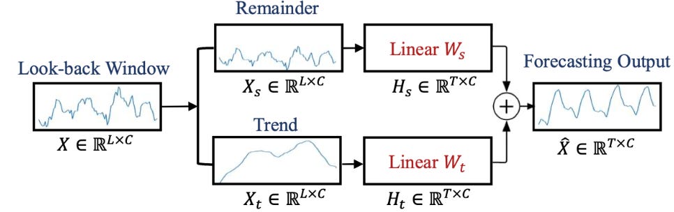
DLinear takes the basic principles of forecasting and applies a clever yet straightforward approach to outshine some Transformer-based models in specific contexts. Concretely, each channel of the time-series input sequence is treated as a whole and provided as input to a simple model (e.g., linear transformation):

Linear prediction for time series. Source: [7].

DLinear also proposes a decomposition strategy with linear layers, borrowed from models like Autoformer and FEDformer. Here’s how it works:

Decomposition: DLinear first decomposes the raw input time series into two components—trend and remainder (seasonal)—using a moving average kernel. This decomposition helps the model handle complex time-series data in a way that emphasizes the long-term trend and seasonal fluctuations separately.
Two Linear Layers: After decomposition, DLinear applies two separate one-layer linear models to each component (trend and seasonal). By doing so, it captures both the long-term trend and the short-term seasonality in a very efficient manner.
Combining the Components: Finally, the outputs of the trend and seasonal models are summed up to produce the final forecast.

👀 The model also has a variant, NLinear, designed to handle dataset distribution shifts. NLinear normalizes the input by subtracting the last value of the sequence, passing it through a linear layer, and then adding the subtracted value back.

The experiments reveal that DLinear and its variants show competitive performance against complicated Transformer-based methods:

❌ One obvious limitation of DLinear is that it treats each channel independently, which may ignore the correlations across variates that may be beneficial for forecasting.

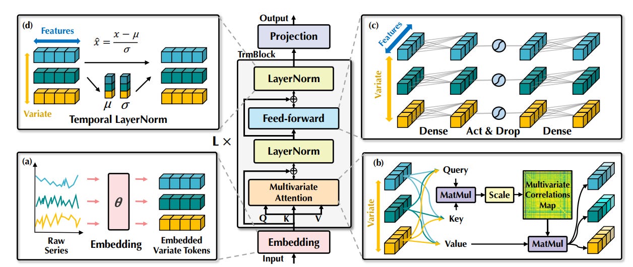
👉iTransformer: A Step Beyond DLinear [8]

This work addresses the limitations of Transformers :

❌Falter with multivariate time series, compressing data at timestamps and losing crucial inter-variate correlations.

❌ The attention mechanisms also struggle with temporal dependencies.

iTransformer offers a solution by inverting the approach. It treats each variate as an independent token, allowing the attention mechanism to directly capture relationships between variates. This variate-centric view enables the model to effectively learn complex dependencies, leading to more accurate and robust time series forecasts. By shifting the focus from timestamps to variates, iTransformer unlocks a powerful new way to understand and predict time series data.

To this end, iTransformer uses DLinear to process temporal steps and Transformer’s attention to model channel relationships:

👉TimeMixer: A Multiscale Approach for Time Series Forecasting [9]

The TimeMixer method is designed to leverage the multiscale nature of time series data, where different scales exhibit unique properties. By focusing on modeling time-series specialty, the paper can achieve good results even without any attention mechanism.

To begin, TimeMixer first downsamples the input time series X into multiple scales using average pooling:

\(X = \{x_0, x_1, \dots, x_M\}, \quad x_m \in \mathbb{R}^{\left\lfloor \frac{P}{2^m} \right\rfloor \times C}, \quad m \in \{0, 1, \dots, M\} \)

where x₀ is the finest scale, and x_M is the coarsest scale.

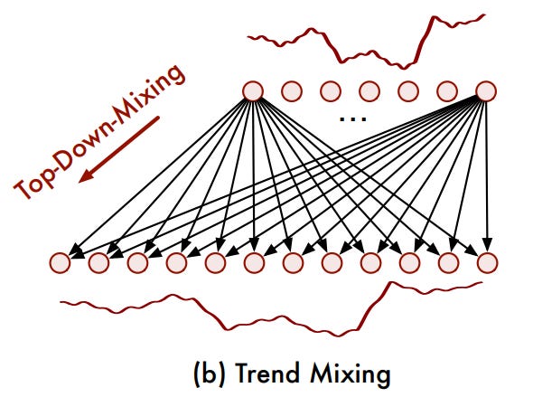
In TimeMixer, the past information is processed using stacked Past-Decomposable-Mixing (PDM) blocks. The core idea behind PDM is to separate seasonal and trend components at each scale and mix them separately across scales.

Decomposition:

\( s_l^m, t_l^m = \text{SeriesDecomp}(x_l^m), \quad \forall m \in \{0, 1, \dots, M\} \)

Seasonal Mixing: In seasonal mixing, the paper uses a bottom-up approach to incorporate finer-scale data, enhancing the modeling of coarser scales and emphasizing the importance of detailed information for seasonal prediction.

\(\text{for } m: 1 \to M, \quad s_l^m = s_l^m + \text{Bottom-Up-Mixing}(s_l^{m-1})\)

Trend Mixing: In contrast to seasonal components, detailed variations in trend data can introduce noise when capturing broader trends. Coarser scale time series offer clearer macro-level information than finer scales. Thus, they use a top-down mixing approach to leverage macro-level insights from coarser scales to guide trend modeling at finer scales.

\(\text{for } m: (M-1) \to 0, \quad t_l^m = t_l^m + \text{Top-Down-Mixing}(t_l^{m+1}) \)

Seasonal and Trend Mix:

\(X_l = X_{l-1} + \text{FeedForward} \left( S\text{-Mix} \{s_l^m\}_{m=0}^M + T\text{-Mix} \{t_l^m\}_{m=0}^M \right) \)

The final prediction just combines prediction at all scales:

👉CycleNet: Leveraging Explicit Periodic Modeling for Long-Term Time Series Forecasting [11]

CycleNet introduces a novel approach to improve long-term time series forecasting by explicitly modeling periodic patterns present in the data. The core of CycleNet lies in its Residual Cycle Forecasting (RCF) technique, which decomposes the time series into periodic components and residuals. The residuals, representing the fluctuations that cannot be explained by periodic patterns, are then predicted to complete the forecast. This approach offers a clear distinction between cyclic and non-cyclic components.

Given a time series with D channels and a cycle length W, the goal is to model the inherent periodicity within each channel. This is achieved through learnable recurrent cycles, denoted by Q∈R^WxD, initialized to zero and trained to represent the cyclic components of the sequence. Some key points:

These recurrent cycles are globally shared across channels
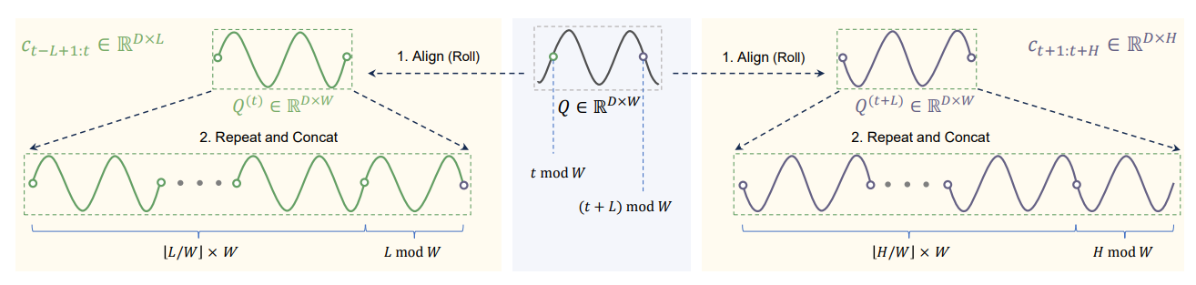
The process of modeling the periodic patterns involves cyclic replications of the recurrent cycles to match the length of the input sequence.

For an input x_t-L+1:t the corresponding cyclic components c_t-L+1:t(past) and c_t+1:t+H(future) are generated by shifting and repeating the recurrent cycles Q as follows:

Shift Q by t mod W positions to get Q(t), where t mod W represents the relative position of the current sequence within Q.
Repeat Q(t) ⌊L/W⌋ times and concatenate the first L mod W elements of Q(t).

Cycles generation. Left is for past data and right is for future data. Source: [11].

Given the cycles, we make predictions by:

Subtract the past cycle from the original time series to get the residual
Given past residual, predict the future residual
Reconstruct the future time series by adding the future residual with the future cycles

CycleNet Prediction with *D=3*. Source: [10].

Despite its simplicity, the method exhibits very good performance on standard time series benchmark:

That said, there are unavoidable limitations:

❌ This approach assumes that cyclic patterns with constant cycle length exist in the time series. The unit cycle length W must be pre-defined.

❌ Similar to DLinear, it does not model cross-channel relationships.

👉SOFTS: A Simple, More Efficient Time-Series Forecaster [12]

The new approach offers a fresh take on time-series forecasting that ditches the heavy attention mechanisms in favor of a lightweight MLP-based approach. Instead of treating each channel independently (losing useful correlations) or relying on expensive attention layers, SOFTS finds a sweet spot: it first extracts a global "core" representation of the time series and then fuses this core back into individual channels.

Concretely, there are 4 steps:

Embedding the Time Series: Each channel is projected into a hidden space of dimension d using a linear embedding function.

\(S_0 = \text{Embedding}(X), \quad S_0 \in \mathbb{R}^{C \times d} \)

Here, C is the number of channels.

Channel Interaction via STAR: The STAR module refines the channel representations over multiple layers. Instead of direct pairwise interactions, STAR aggregates information into a core representation:

\(o = f(s_1, s_2, \dots, s_C) \)

STAR's idea is to model channel interaction as a centralized representation. Source: [12].

Concretely, at iteration/layer i, the method computes the function f as:

\(o_i = \text{StochPool}(\text{MLP}_1(S_{i-1})) \)

Here, Stochastic pooling (StochPool) aggregates representations from C series by randomly selecting values, effectively blending the characteristics of mean and max pooling.

Fusing Core and Channel Representation

The core representation is concatenated with each channel.

\(F_i = \text{Repeat_Concat}(S_{i-1}, o_i) \)

The fused representation is then projected back to the hidden space with a residual connection:

\(S_i = \text{MLP}_2(F_i) + S_{i-1} \)

Prediction Layer:

MLP takes the fused representation to make predictions:

\(\hat{Y} = \text{Linear}(S_N), \quad \hat{Y} \in \mathbb{R}^{C \times H} \)

We can summarize the steps in the diagram below:

Series-cOre Fused Time Series forecaster (SOFTS). Source: [12].

The results are impressive compared to prior works including Transformer-based methods:

Conclusion

Time-series forecasting remains one of the most challenging problems in AI, demanding models that can capture complex temporal dependencies, handle non-stationarity, and generalize across diverse patterns. Unlike standard machine learning tasks, time-series data is sequential, highly dynamic, and often influenced by external factors, making it resistant to one-size-fits-all solutions.

The Road Ahead: The increasing demand for long-range forecasting, adaptation to distribution shifts, and better uncertainty quantification calls for innovations beyond current architectures. One promising direction is the integration of Large Language Models (LLMs) into time-series forecasting, leveraging their pretrained knowledge and ability to process complex dependencies and adapt to diverse forecasting tasks.

🔥 Coming Next: In my next blog, I’ll explore how LLMs can be adapted as a new solution for time-series forecasting. Stay tuned! 🚀

References

[1] Shi, Xiaoming, Shiyu Wang, Yuqi Nie, Dianqi Li, Zhou Ye, Qingsong Wen, and Ming Jin. "Time-moe: Billion-scale time series foundation models with mixture of experts." ICLR, 2025.

[2] Shumway, Robert H., David S. Stoffer, Robert H. Shumway, and David S. Stoffer. "ARIMA models." Time series analysis and its applications: with R examples (2017): 75-163.

[3] Holt, C. C. (1957). Forecasting seasonals and trends by exponentially weighted averages (O.N.R. Memorandum No. 52). Carnegie Institute of Technology, Pittsburgh USA.

[4] Wu, Haixu, Jiehui Xu, Jianmin Wang, and Mingsheng Long. "Autoformer: Decomposition transformers with auto-correlation for long-term series forecasting." Advances in neural information processing systems 34 (2021): 22419-22430.

[5] Zhou, Tian, Ziqing Ma, Qingsong Wen, Xue Wang, Liang Sun, and Rong Jin. "Fedformer: Frequency enhanced decomposed transformer for long-term series forecasting." In International conference on machine learning, pp. 27268-27286. PMLR, 2022.

[6] Nie, Yuqi, Nam H. Nguyen, Phanwadee Sinthong, and Jayant Kalagnanam. "A time series is worth 64 words: Long-term forecasting with transformers." arXiv preprint arXiv:2211.14730 (2022).

[7] Zeng, Ailing, Muxi Chen, Lei Zhang, and Qiang Xu. "Are transformers effective for time series forecasting?." In Proceedings of the AAAI conference on artificial intelligence, vol. 37, no. 9, pp. 11121-11128. 2023.

[8] Liu, Yong, Tengge Hu, Haoran Zhang, Haixu Wu, Shiyu Wang, Lintao Ma, and Mingsheng Long. "iTransformer: Inverted Transformers Are Effective for Time Series Forecasting." In The Twelfth International Conference on Learning Representations.

[9] Wang, Shiyu, Haixu Wu, Xiaoming Shi, Tengge Hu, Huakun Luo, Lintao Ma, James Y. Zhang, and JUN ZHOU. "TimeMixer: Decomposable Multiscale Mixing for Time Series Forecasting." In The Twelfth International Conference on Learning Representations.

[10] Qiu, Xiangfei, Jilin Hu, Lekui Zhou, Xingjian Wu, Junyang Du, Buang Zhang, Chenjuan Guo et al. "Tfb: Towards comprehensive and fair benchmarking of time series forecasting methods." arXiv preprint arXiv:2403.20150 (2024).

[11] Lin, Shengsheng, Weiwei Lin, Xinyi Hu, Wentai Wu, Ruichao Mo, and Haocheng Zhong. "Cyclenet: enhancing time series forecasting through modeling periodic patterns." Advances in Neural Information Processing Systems 37 (2024): 106315-106345.

[12] Han, Lu, Xu-Yang Chen, Han-Jia Ye, and De-Chuan Zhan. "SOFTS: Efficient Multivariate Time Series Forecasting with Series-Core Fusion." In The Thirty-eighth Annual Conference on Neural Information Processing Systems.

Neurocoder Tales

Discussion about this post