
The Best of Time-Series Forecasting (Part II): Advancements in Time Series Modeling Through Large Language Models
A comprehensive collection of leading LLM papers on time series forecasting

Part 1 of my blog looked at how time-series forecasting has evolved—from traditional models like ARIMA to deep learning methods like Transformers. These approaches brought big improvements, especially in handling complex and long-range patterns. However, they also have limits, especially when it comes to adapting to new data or working well across very different domains.
Now, a new wave of models is entering the scene: Large Language Models (LLMs). These models were originally built for language tasks—like chatbots, summarizing text, and answering questions. But recently, researchers have started using LLMs for time-series forecasting, too.
In this post, we’ll explore:
✔ How LLMs are being adapted to handle time-series data
✔ Some recent research and early results
✔ Key challenges and open questions
LLMs won’t replace every forecasting model, but they’re opening up new ideas about how we can approach time-series problems. Let’s take a look at where this is all heading.

Table of Contents
Why Do We Need Large Language Models?
Time-series forecasting has been a long-standing challenge in data science, underpinning critical applications like financial market prediction, weather forecasting, and supply chain management. For the last 30 years, statistical models such as ARIMA and ETS have been extensively used for time-series tasks, followed by deep learning methods like LSTMs and Transformers. So, why are researchers now turning to Large Language Models (LLMs) for time-series forecasting?
Pattern Recognition Capability
LLMs excel at recognizing complex patterns across diverse data sources, including both structured numerical sequences and unstructured text. Their self-attention mechanism allows them to capture long-range dependencies and underlying trends in time-series numbers. For example, big LLMs like ChatGPT can find the number patterns easily:

Understanding Context Beyond Numbers
Additionally, LLMs can leverage their pre-trained knowledge to identify contextual signals—such as economic shifts, seasonal effects, or market sentiment—helping to enhance time-series forecasting beyond traditional statistical and deep learning approaches.
Long-term Forecasting
While traditional time-series models learn patterns from past data, they often struggle with long-term dependencies. LLMs, especially those equipped with long-term memory architectures, can store and recall historical insights more effectively, improving their ability to recognize seasonality, anomalies, and evolving trends over time.
👀 That said, since LLMs are primarily designed for text data, applying them to time-series data is not straightforward. In the following sections, we will explore recent works that address this challenge.
Direct Application of Pre-trained LLMs
A key approach is converting numerical time-series data into text, representing each value as a string, i.e., prompt-based forecasting. Because the sequence order is maintained in string form, LLMs can still capture temporal dependencies. Here, the choice of tokenization is crucial, as it determines how the model processes and learns patterns from the data.
Several notable examples illustrate the direct prompting approach. 👉PromptCast [1] represents a pioneering effort in this direction, converting numerical time series into natural language prompts using predefined templates. This framework frames the forecasting task as a sentence-to-sentence generation problem, where the LLM is prompted with historical data described in natural language and asked to generate a sentence representing the forecast.
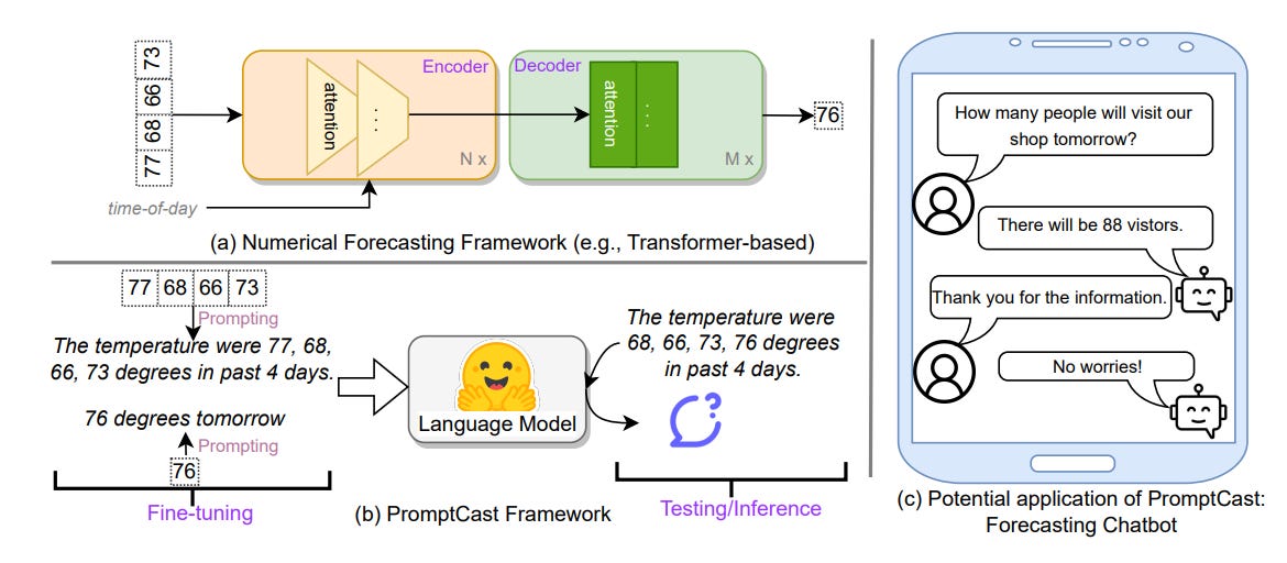
The paper introduces simple templates to translate time series to prompts. For example, for the ECL dataset:

Despite being simple, the approach shows reasonable results compared to other deep learning methods, such as Autoformer and FEDFormer:

👀 The paper only uses small and old LLMs such as BigBird and Pegasus. The results can be even better with stronger and modern LLMs such as Chat-GPT.
Unlike PromptCast, which focuses on prompt engineering, the 👉LLMTime [2] paper demonstrates that LLMs can be used directly as forecasters without the need for additional text or prompt engineering, provided that the numerical values are carefully preprocessed.
For example, the choice of tokenization (with space or not) matters:

In particular, the paper proposes:
Digits are spaced out for separate tokenization.
Commas mark time steps.
Decimal points are removed to save context (e.g., by multiplying the original value with 100)
Example: 0.123, 1.23, 12.3, 123.0 → "1 2 , 1 2 3 , 1 2 3 0 , 1 2 3 0 0"
Other tricks include:
Rescaling: The method rescales time series values so that the α-percentile of the rescaled data is 1, preventing extreme values from dominating while ensuring the LLM sees some examples where digit lengths change. For example, a time series has values
[10, 50, 200, 1000], and we set α = 0.75. If the 75th percentile value is 200, we scale all values by 1/200, so the rescaled series becomes[0.05, 0.25, 1, 5],Sampling: To forecast, generate multiple samples (e.g., 20) from the LLM and use their statistics (e.g., median or quantiles) to create a point or probabilistic estimate.
Likelihood Estimation: To get good sampling, the paper refines the way to compute the probability of the LLM’s output. The approach allows LLMs to act like hierarchical softmax distributions over numerical values. A number u of n digits has probability:

To estimate the probability for a “continous“ value x by assigning a uniform probability within the bin that x falls into. For example, if x=0.5371 falls into bin k (0.537-0.538):
where B is the number base, e.g, B=10, each bin has the probability B⁻ⁿ.
The experiment results demonstrate that LLMTime is competitive against standard and deep forecasting methods:

LLMs are showing promise in time-series forecasting, but basic prompting limits them. A more recent work, 👉LSTPrompt, introduces a sophisticated Chain-oj-Thought prompt to break down forecasting, improving accuracy.
Some prompting techniques:
Add task description
Explain the long-term/short-term properties of the data
Include “TimeBreath” trick prompt

Despite promising results, directly using LLMs “as-is“ for time-series forecasting has key limitations:
❌ No temporal inductive bias: LLMs lack built-in mechanisms for capturing time dependencies.
❌ Tokenization artifacts: Discretization may reduce numerical precision.
❌ High computational cost: More expensive than traditional models.
❌ Limited extrapolation: Struggles with long-term forecasts.
❌ Lack of domain constraints: Misses explicit trend/seasonality modeling.
In the next section, we will see more complicated solutions that address these concerns.
❌ High cost: Good results often require strong LLMs as GPT-4. However, this is expensive and not open-source.
Designing and Fine-tuning LLMs for Time Series Forecasting
To overcome these limitations, research has focused on repurposing and fine-tuning LLMs for time-series forecasting. This includes adapting their architecture and further training pre-trained models on time-series data.
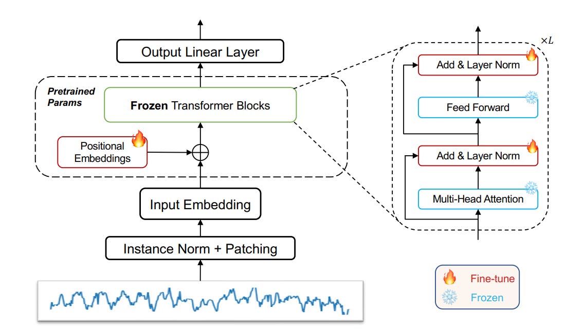
One core technique is aligning the modalities of time series and language, making LLMs effective for time-series data. The obvious way is to choose some early layers of the LLMs to finetune on time-series forecasting tasks to align the encoding part of the LLMs to the time-series domain. For example, GPT4TS [4] only finetunes positional embeddings and layer normalization parts of the GPT model:
Similarly, 👉LLM4TS [7] develops an LLM framework for time-series forecasting. Compared to GPT4S, more engineering effort is spent on timestamp and time-series embedding to represent the tokens for the LLM engine. For example, the paper proposes to embed each time scale information separately with a final pooling to get the temporal representation etemp:

Then, the final embedding is computed as:
where etoken is the time-series patch representation and epos is the positional encoding.
The paper also introduces a two-step training approach:
Alignment training, where the model learns to align representations through a next-token prediction task, similar to the pretraining phase in LLMs;
Forecasting fine-tuning, where the model is further trained on downstream time series forecasting tasks to specialize in prediction.

👀 Although these methods aim to align LLM text representations with time series data, they largely stop at simply retraining the encoding layers without deeper adaptation.
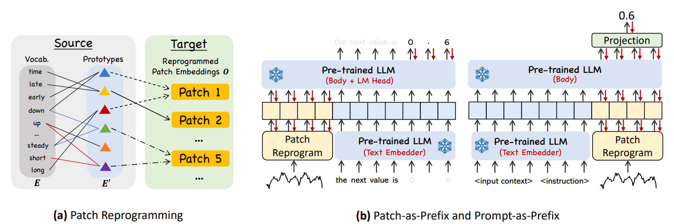
Digging deeper, 👉Time-LLM [5] exemplifies a reprogramming framework where the input time series is transformed into text prototype representations and natural language prompts are used to guide the LLM's reasoning process. This approach keeps the underlying LLM intact and trains a separate reprogramming layer to translate the observed time series into a language-based representation, as illustrated in Fig. c below:

👀Essentially, reprogramming framework finetunes the model's input and output layers while keeping its core frozen for efficiency.
Here, the paper proposes patch reprogramming to align time series with the LLM’s embedding space by transforming a subsequence of time series (patch) to a text-aligned token representation. As such, they start with pretrained embedding of text tokens:
where V is vocabulary size and D is embedding dimension. Direct mapping is inefficient, they propose to project the original embedding space to a smaller prototype space E’:
These prototypes encode phrases like "short up" or "steady down", keeping representations within the LLM’s text space, yet more specific. Then, they integrate prototypes to time-series representation via cross-attention. For an attention head k, the query Q is constructed from the time-series patch Xp while the key and value are generated from the prototype embedding:
The attention mechanism computes the alignment between a patch (i) and prototypes:
Aggregating across heads produces the reprogrammed representation, which is then linearly projected to match the hidden dimensions of the backbone model:
Given the reprogrammed patches, the paper proposes 2 ways to feed them to the LLMs:
Patch-as-Prefix: Treat patch as input text followed by a simple prompt to trigger the LLM to predict time series values in natural language. However, this method faces challenges:
LLMs struggle with high-precision numerals without external tools, making long-horizon forecasting difficult.
Different pre-training corpora and tokenization strategies lead to inconsistencies in representing numeric values (e.g.,
['0', '.', '6', '1']vs.['0', '.', '61']).
Prompt-as-Prefix circumvents these limitations by structuring prompts with three key components:
Use instruction prompt as input context, task instruction, and trends and lags statistics.
The instruction precedes the patch, and we extract only the output segment corresponding to the patch for regression, similar to standard forecasting. A projection layer is needed to align the output.
With these architecture changes, the performance on long-term forecasting tasks is impressive:

Given these results, it seems that LLMs will have huge potential for boosting forecasting accuracy. However, a recent study [6] reveals that it is not that easy. The research question is: 👉Are Language Models Actually Useful for Time Series Forecasting?
The finding shows that:
Despite the hype, large language models (LLMs) don’t help with time series forecasting—in fact, simpler models without LLMs often perform better.
LLMs add extra cost without improving accuracy, struggling to understand time-based patterns, or helping in low-data situations.
To understand why, let’s look at the experimental setting:

Here, the paper considers the standard architecture of utilizing LLMs for forecasting tasks, which may involve a pre-trained LLM and other components:
Input normalization
Finetune encoding and projection layers
Alignment training
To confirm the contribution of the LLM component, the paper removes or replaces the LLM module with other things. It turns out that without the LLM module, the performance tends to be better:

👀 The results suggest that improvements in previous papers is mainly attributed to normalization and encoding layer finetuning.
More results confirm that the pre-training knowledge stored in LLMs may not be useful for forecasting tasks. As shown below, even without using pre-training weights, the model can still perform best.

👀 Althouth the result is interesting, it is only tested on GPT-2, a weak LLM. It does not guarantee for other LLMs.
If LLMs do not help, 🧠where does the performance come from? The paper suggests that simple techniques used in current LLM forecasters are enough to build strong forecasters:
Patching (channel independent)
One-layer attention
Linear projections

If this finding sounds grim for the future of LLMs in time series, there’s good news: a recent study shows that when used the right way, LLMs can significantly boost forecasting performance. It’s not that LLMs are useless—it’s that how we use them makes all the difference.
Concretely, most existing LLM-based time series models miss a key ingredient: autoregression—the core of how both LLMs and traditional forecasters make predictions. A new approach, 👉AutoTimes [8], brings this back by using LLMs in their natural autoregressive mode, enabling flexible, multi-step forecasts without needing to retrain for different input/output lengths.
AutoTimes leverages existing components and ideas:
Patching to encode a segment of a time series as a token representation
Timestamp representation modeling to improve token representation
Only 0.1% of parameters are added by embedding time series as LLM tokens—keeping the LLM frozen and training efficient.
The main contribution here is that it trains the LLMs with autoregression style with the next token prediction task. The predicted tokens are then projected back to time-series space for forecasting:

Under this approach, the results look promising:

More importantly, the paper shows that the LLM module is really useful, as indicated in the ablations study:

We can see that by designing the right method for LLMs, their full potential in time series forecasting can finally be unlocked. With approaches like AutoTimes, LLMs go beyond being just expensive add-ons—they become efficient and generalizable forecasters.
Building Foundational Models for Time Series: A New Era?
Instead of just adapting existing LLMs, researchers are now exploring specialized foundational models trained directly on vast time series data.
Why Specialized Models? Training LLMs from scratch on time series could help them understand temporal dependencies just as language models learn from text.
Challenges & Breakthroughs: Time series data is highly variable and non-stationary, making dataset creation and training complex, but models like TimeGPT and Chronos show it's possible. Let’s discover how these specialized LLMs are reshaping time series forecasting.
👉TimeGPT [9], the first time-series foundation model, employs Transformer architecture to learn time-series representations. It processes a sliding window of historical values, enriched with local positional encodings, and passes this through a deep encoder-decoder stack with residual connections and layer normalization. At the end, a linear head maps the decoder’s output to a forecasting window—predicting what comes next. The training objective is:
The paper applies Transformer-based architecture on time-series datasets:

👀 TimeGPT is not based on an existing language model. While it shares the “foundation model” spirit—training on vast data at scale—its architecture is customized for numerical sequences, not text.
To train TimeGPT, researchers compiled what’s likely the largest public collection of time series ever used, with over 100 billion data points. This dataset spans a rich mix of domains: finance, economics, healthcare, demographics, weather, web traffic, transport, IoT sensors, and more. These series bring with them a wide spectrum of behaviors—multiple seasonalities, varying cycle lengths, non-linear trends, noise, and sudden anomalies.
👀 Instead of overly sanitizing the data, the creators kept most of it raw, simply standardizing formats and filling in missing values. This decision ensured the model would learn from real-world messiness—a critical factor in achieving robustness and generalization.
Training TimeGPT required multiple days on NVIDIA A10G GPU clusters. Extensive tuning was conducted to optimize batch sizes, learning rates, and other parameters. Consistent with earlier large-scale training studies, larger batch sizes, and smaller learning rates helped stabilize training.
One standout feature of TimeGPT is its support for probabilistic forecasting—not just predicting what’s most likely to happen, but quantifying uncertainty around those predictions. This is achieved using conformal prediction, a model-agnostic, non-parametric method that doesn’t assume a specific distribution. During inference, TimeGPT performs rolling forecasts on the latest data to estimate and calibrate the model’s prediction intervals, making it a more trustworthy tool for decision-making under uncertainty.
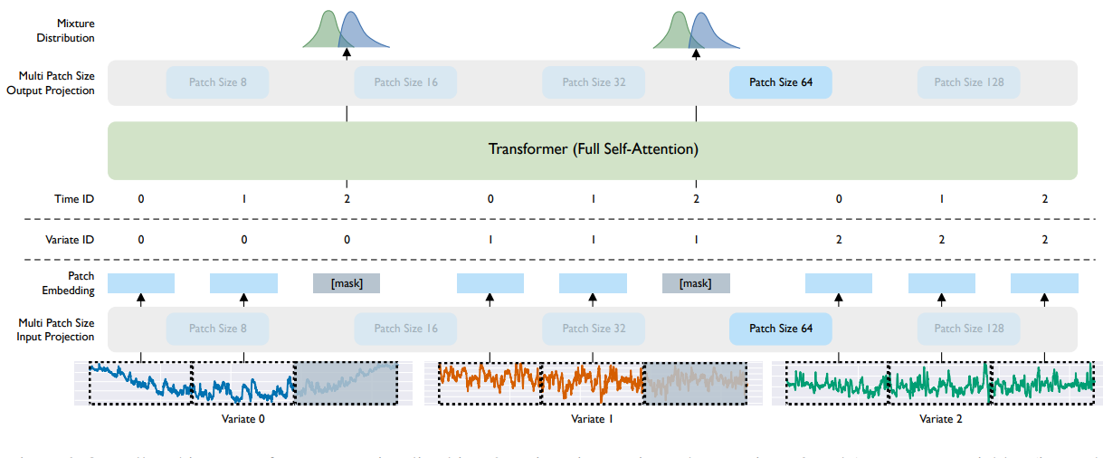
Sharing the same spirit with TimeGPT, 👉MOIRAI [10] prepares a large-scale time-series dataset and trains a Transformer-based model with the data. However, MOIRAI provides more sophisticated encoding and decoding pipelines. First, it proposes a Patch-based Masked Forecasting framework where it divides time series into non-overlapping patches and learns to forecast the masked future patches using a Transformer encoder.
Each patch captures temporal chunks of data, and multiple patch sizes are used to adapt to both high- and low-frequency signals.
During training, future patches are replaced with a special
[mask]token — a learnable embedding — signaling the model to predict them.
Most models assume fixed-length multivariate inputs. MOIRAI aims to work with any number of variates, even if unseen during training. To this end, it flattens multivariate time series into a single long sequence and applies attention to it. To preserve variate identity and ensure robustness to variate permutation:
It uses variates encodings (not positional encodings).
Applies binary attention biases that help the Transformer:
Distinguish between intra- and inter-variate interactions.
Remain equivariant to variate order and invariant to variate IDs.
In particular, define the rotary positional encoding matrix as R and let u(1), and u(2) be learnable scalars, we have the attention score:
Here, the binary attention bias is controlled by u as the two scalars bias the attention scores based on whether the variate (m,n) indices match:
u(1) enhances attention between elements of the same variate.
u(2) modulates cross-variate attention.
They are learned to best fit the training data. The final attention weights are:
MOIRAI adopts several modern LLM techniques to stabilize and improve the Transformer encoder:
RMSNorm replaces LayerNorm
SwiGLU activation used in FFNs
Query-key normalization for attention
Pre-normalization layout for better gradient flow
Biases are removed for simplicity and regularization
Finally, instead of predicting a single value, MOIRAI outputs parameters of a mixture of parametric distributions — allowing flexible and accurate uncertainty modeling. In particular, the output reads:
Here, Yt:t+h is the time-series patch. Distribution choices:
Student’s t – for general robustness
Negative Binomial – for count-based data
Log-normal – for right-skewed distributions (e.g., prices)
Low-variance Normal – for high-confidence predictions
This setup supports both sampling and likelihood-based training with minimal overhead. The loss function represents the negative log-likelihood:
The whole pipeline is given below:
In terms of performance, MORAI can outperform some deep learning forecasters. This is remarkable because the foundation model does not train on each dataset as the other baselines.

Approaching differently, 👉Chronos [11] repurposes standard language models—like T5 or GPT-2—to handle time series data with minimal changes, by converting continuous time series values into discrete tokens. These tokenized sequences are then treated as a “language of time series” that LMs can ingest and model.
To make time series digestible for LLMs:
Scaling: Each time series is normalized, particularly via mean scaling (preserving zero values, e.g., "zero sales" days).
Quantization: The scaled values are mapped to discrete bins (e.g., 1024 total). They use uniform binning (equal bin widths) to generalize better across unseen data distributions.

👀 This converts a real-valued time series into a discrete sequence:
[x1, ..., xC] → [token1, ..., tokenC].This is similar to fine-tuning LLM approaches mentioned above.
Then, the LLMs are employed to process the data
Off-the-shelf LMs (like T5 or GPT-2) are used without architecture changes.
Only modification: Adjusting vocabulary size to match the quantized token space.
No time or frequency features (e.g., no day-of-week encoding), which surprisingly doesn’t degrade performance.
The training Objective is the standard cross-entropy loss over the token vocabulary:
Predicts next token zC+h+1 given previous tokens z1:C+h
Trained like standard language modeling

During inference, Chronos samples token autoregressively:
These tokens are dequantized and unscaled back to real numbers.
Multiple samples are drawn to get probabilistic forecasts, forming a distribution over possible futures.
Chronos tackles the data scarcity problem with two strategies:
TSMixup – Combines time series from different datasets via convex interpolation.
KernelSynth – Uses Gaussian processes to generate synthetic time series with random kernel compositions.
These data augmentation techniques improve generalization and robustness, especially for zero-shot settings.
Chronos was trained and evaluated across 55 datasets and:
Outperformed traditional time series models and specialized deep nets.
Achieved state-of-the-art zero-shot performance—i.e., good generalization without fine-tuning, i.e., better than MORAI.
Performed competitively even with modest model sizes, making it computationally efficient.
The benchmark mainly involves 2 metrics:
WQL evaluates the accuracy of probabilistic forecasts (i.e. when your model predicts a distribution or multiple quantiles, not just a single value).
MASE is a scale-independent metric used to evaluate point forecasts. It compares your forecast to a naive baseline (like the previous value or seasonal naive).

While models like Chronos and Moirai have made notable progress towards universal forecasting, they face limitations:
❌ They rely on moderate and fixed context lengths or handcrafted heuristics that limit their flexibility and scalability.
❌ They follow dense training, i.e., being computationally expensive and requiring large GPUs to accommodate.
To address these issues, researchers recently introduced 👉TIME-MoE [12]—a scalable, sparse, and general-purpose time series foundation model built to mirror the success of LLMs and vision transformers in their respective domains. In particular, the model features:
Decoder-only Transformer with a Mixture-of-Experts (MoE) backbone.
Operates in an auto-regressive manner, enabling support for any forecasting horizon.
Capable of handling long contexts (up to 4096 tokens), which is critical for long-term temporal dependencies.
Sparse activation: Only a tiny subset of expert networks are activated per token, making the model highly efficient.
Allows the model to scale up (up to 2.4 billion parameters) without linear increases in compute cost.
Below is the overall architecture and details of each processing step.

①② The first step is to embed time series data into tokens. Unlike the mainstream that uses patch-based tokenization, here they use point-wise tokenization, i.e., each time-series step is projected to high-dimensional embedding:
where:
W and V are learnable projection weights
⊗ denotes element-wise product
③ TIME-MoE builds on the decoder-only transformer, with common tricks for time series:
RMSNorm for stable training
Rotary Positional Embedding (RoPE) to better generalize to long-range sequences
Bias-free Layers (except in self-attention) for better extrapolation
The twist: each transformer block replaces the standard feedforward layer with a Mixture-of-Experts module. Here's what happens at a layer l step-by-step:
i. Self-Attention + Residual:
ii. Normalization:
iii. Mixture-of-Experts Activation:
In this step, the Mixture layer routes each token to a subset of K out of N possible experts, plus a shared expert to capture global knowledge:
Where the gating weights gi,t are determined via softmax over router scores si,t. In particular, the gating weights for each specialized expert are:
with the router’s score is computed as:
On the other hand, the gate for the global expert is:
④⑤ Another contribution of the approach is that instead of predicting at a single horizon, TIME-MoE predicts at multiple resolutions simultaneously. Each projection head targets a different forecast length, enabling the model to:
Generalize across short and long horizons
Learn a richer latent structure of the future
Ensemble multi-scale predictions for better robustness
The total loss averages over all resolutions, using the Huber loss for each prediction:
Last but not least, MoE models suffer from a known issue: routing collapse, where only a few experts get chosen repeatedly. To fix this, TIME-MoE introduces an auxiliary expert balance loss:
where fi is the fraction of tokens routed to expert i:
ri is the average router probability for expert i:
👀 Minimizing the balance loss encourages uniform expert assignment. This is because the frequency f and the routing vector r are positively correlated (i.e., approximately proportional), allowing us to apply Chebyshev’s sum inequality.
The result is impressive. Time-MOE is now one of the SOTA in time-series forecasting when compared with other foundation models:
as well as other specialized methods:
Conclusion
LLMs aren’t the final answer to time-series forecasting, but they’ve changed the conversation. What started as a tool for language tasks is now being reimagined for sequences of all kinds. Researchers are finding creative ways to adapt pre-trained LLMs to time-series problems, fine-tune them for specific domains, or even build new foundational models trained purely on temporal data. Some of these early results are promising.
The takeaway? LLMs are giving us a new lens on forecasting problems. They open up ideas that weren’t obvious before—ideas about scale, transferability, and reasoning over time. That doesn’t mean we throw out everything we’ve learned from classical and deep learning models. It just means we now have another tool to work with—and a new frontier to explore.
Reference
[1] Xue, Hao, and Flora D. Salim. "Promptcast: A new prompt-based learning paradigm for time series forecasting." IEEE Transactions on Knowledge and Data Engineering 36, no. 11 (2023): 6851-6864.
[2] Gruver, Nate, Marc Finzi, Shikai Qiu, and Andrew G. Wilson. "Large language models are zero-shot time series forecasters." Advances in Neural Information Processing Systems 36 (2023): 19622-19635.
[3] Liu, Haoxin, Zhiyuan Zhao, Jindong Wang, Harshavardhan Kamarthi, and B. Aditya Prakash. "LSTPrompt: Large Language Models as Zero-Shot Time Series Forecasters by Long-Short-Term Prompting." In Findings of the Association for Computational Linguistics ACL 2024, pp. 7832-7840. 2024.
[4] Zhou, Tian, Peisong Niu, Liang Sun, and Rong Jin. "One fits all: Power general time series analysis by pretrained lm." Advances in neural information processing systems 36 (2023): 43322-43355.
[5] Jin, Ming, Shiyu Wang, Lintao Ma, Zhixuan Chu, James Y. Zhang, Xiaoming Shi, Pin-Yu Chen et al. "Time-LLM: Time Series Forecasting by Reprogramming Large Language Models." In The Twelfth International Conference on Learning Representations, 2019.
[6] Tan, Mingtian, Mike Merrill, Vinayak Gupta, Tim Althoff, and Tom Hartvigsen. "Are language models actually useful for time series forecasting?" Advances in Neural Information Processing Systems 37 (2024): 60162-60191.
[7] Chang, Ching, Wei-Yao Wang, Wen-Chih Peng, and Tien-Fu Chen. "Llm4ts: Aligning pre-trained llms as data-efficient time-series forecasters." arXiv preprint arXiv:2308.08469 (2023).
[8] Liu, Yong, Guo Qin, Xiangdong Huang, Jianmin Wang, and Mingsheng Long. "Autotimes: Autoregressive time series forecasters via large language models." Advances in Neural Information Processing Systems 37 (2024): 122154-122184.
[9] Garza, Azul, Cristian Challu, and Max Mergenthaler-Canseco. "TimeGPT-1." arXiv preprint arXiv:2310.03589 (2023).
[10] Woo, Gerald, Chenghao Liu, Akshat Kumar, Caiming Xiong, Silvio Savarese, and Doyen Sahoo. "Unified Training of Universal Time Series Forecasting Transformers." In International Conference on Machine Learning, pp. 53140-53164. PMLR, 2024.
[11] Ansari, Abdul Fatir, Lorenzo Stella, Ali Caner Turkmen, Xiyuan Zhang, Pedro Mercado, Huibin Shen, Oleksandr Shchur et al. "Chronos: Learning the Language of Time Series." Transactions on Machine Learning Research, 2024.
[12] Shi, X., Wang, S., Nie, Y., Li, D., Ye, Z., Wen, Q., & Jin, M. (2025). Time-MoE: Billion-Scale Time Series Foundation Models with Mixture of Experts. In Proceedings of the Thirteenth International Conference on Learning Representations, 2025.