Reason on the Fly: How RL Boosts LLM Reasoning On the Spot

Surveying New Frontiers in Reinforcement Learning for Language Models (Part 2)

In our last post, we warmed up with why reinforcement learning (RL) is a powerful paradigm for building smarter AI reasoners. Today, we zoom in on an exciting approach: using RL at inference time to improve large language model (LLM) reasoning on the spot. In particular, we explore ways to inject real-time reasoning into static LLMs. Let's break down how RL can transform a frozen LLM into a more dynamic, reasoned thinker at runtime.

Reason on the Fly: How RL Boosts LLM Reasoning On the Spot. Source: OpenAI’s Sora.

Table of Contents

• Why Test-Time Matters

• The First Breakthrough: Test-Time Compute

• Scaling Up Test-Time Efforts

• Process Reward Models: Defining What’s "Good Reasoning"

• Search and Planning with RL

• Conclusion & What’s Next

---

Why Test-Time Matters

A long-standing principle in machine learning is the clean separation between training and inference. Traditional pipelines front-load all the optimization into training, assuming that, once deployed, models will perform inference in a fixed, feed-forward manner. The model learns once and acts passively forever after.

In the context of LLMs, a dominant strategy to improve performance has been simple: scale-up training ⬆️. Larger models, more data, and longer context windows have powered much of the progress to date. And this strategy works until it doesn’t. As we push toward ever-larger scales, we begin to see diminishing returns:

More computing resources are required, but the performance gain is getting smaller. Source: [1]

More parameters don’t necessarily lead to better reasoning. And more data doesn’t guarantee generalization, especially to tasks that are unfamiliar or structurally complex. Why? Because we’re running up against a fundamental bottleneck: the data itself.

As Ilya Sutskever famously put it, “We have but one internet.” That single, finite corpus has already been scraped, filtered, and optimized for training. There is no untapped “second internet” to unlock new capabilities. This saturation of training-time gains is prompting a natural question: 🧠 What else can we optimize?

A new direction is taking shape: test-time compute. Rather than relying solely on what was learned during pretraining, this paradigm focuses on what can be actively computed during inference. The insight is simple but powerful: not all reasoning can (or should?) happen in a single forward pass. Some problems demand more thought. It pays to think longer, search deeper, and adapt on the fly while solving the task.

This idea isn’t new in the broader AI landscape. Fields like robotics, planning, and control have long leveraged test-time optimization to dynamically adjust actions, internal states, or policies based on the current situation. In these domains, the agent doesn’t freeze after training. It continues to optimize in real-time, guided by the specifics of the environment or task at hand. 🧠 So why hasn’t this philosophy fully carried over to LLMs?

Because LLMs are typically treated as static predictors. Once trained, they produce outputs via greedy decoding or sampling, which is efficient, but fixed. This works fine for fluent language generation. Without a mechanism to adapt at test time, LLMs tend to default to surface-level heuristics, even when the task demands deeper computation. This is where test-time reinforcement learning shines as a promising bridge between passive prediction and active, deliberative reasoning.

---

The First Breakthrough: Test-Time Compute

As pretraining-driven gains begin to plateau, the field has turned to post-training methods to push LLM capabilities further. Techniques like alignment through RLHF and instruction tuning have become standard tools to refine behavior after pretraining. But another powerful and increasingly relevant direction is emerging: test-time compute (TTC).

Instead of relying solely on what was baked in during pretraining, TTC explores what a model can compute on the fly, at the moment of inference. What if reasoning didn’t stop when training ended? What if, during deployment, models could think longer, adapt dynamically, and search more strategically to solve hard problems?

This shift in mindset is already underway. OpenAI’s o1 models mark a pivot toward deeper inference-time reasoning:

o1-series “think“ longer and slower. Source.

👀 While the exact techniques remain undisclosed, OpenAI has stated that o1 is “trained with reinforcement learning to perform complex reasoning” [2]. The role of RL is indisputable.

The result is amazing:

o1 models achieve remarkable results on reasoning benchmarks. Source: [2].

• On Codeforces, o1 ranks in the 89th percentile—an unprecedented level of programming ability for a language model.

• On AIME, a prestigious U.S. math competition, o1 ranks among the top 500 students.

• On GPQA, a benchmark of PhD-level science questions, o1 surpasses human experts in physics, chemistry, and biology.

The results reveal a compelling insight: allocating more computational resources at test time by allowing the model to perform multiple reasoning passes, search over alternatives, or optimize responses can yield improvements comparable to, or even surpassing, those from scaling training-time compute:

Performance scaling with train-time and test-time compute. Source: [2].

👀 While the compute costs may appear similar in magnitude, they reflect fundamentally different trade-offs. Training-time compute is a one-time, centralized investment that doesn’t directly affect the end-user experience. In contrast, test-time compute occurs during inference and consumes resources every time the model is used, placing a computational burden on the user or deployment system.

These achievements aren’t just about language. They reflect System 2 reasoning: deliberate, multi-step, and strategic. Unlike System 1, which governs fast, automatic responses like language completion or basic recall, System 2 engages when tasks demand controlled, sequential thinking, such as solving a math proof, writing code, or evaluating competing hypotheses. A summary of System 1 and System 2 properties is given below:

System 1 vs System 2 Overview. Source.

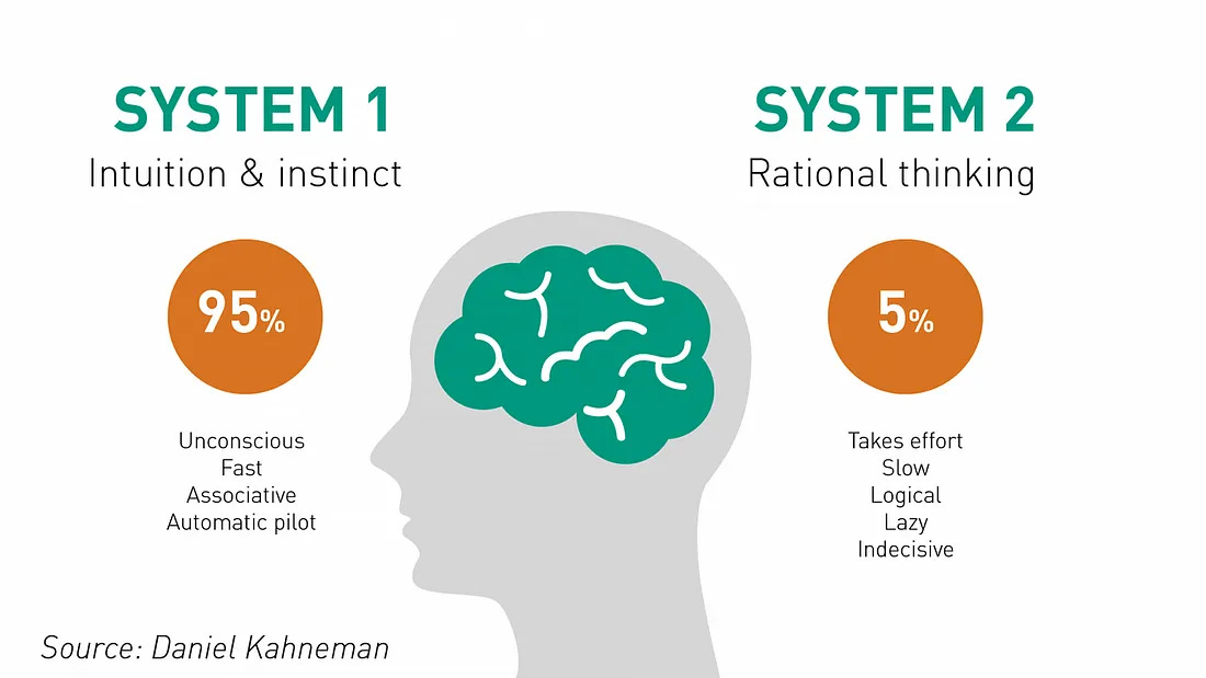
As we can see, System 2 is more powerful with deliberate reasoning. However, this deeper reasoning comes at a cost. High TTC is expensive, making such models suitable only for a narrow slice of high-stakes or compute-rich applications.

This raises two pressing research questions:

1. 🧠 How can we equip LLMs with the ability to scale their test-time reasoning?
   More forward passes? Search over reasoning chains? External tools? Many strategies exist, but Reinforcement Learning (RL) offers a particularly principled framework.

2. 🧠 More importantly, how can we make TTC efficient? Inference-time RL can guide the search process efficiently. Rather than brute-force reasoning, models can learn when and how to allocate extra thinking time for prioritizing hard problems, rethinking weak outputs, or dynamically adjusting their decoding strategy.

We can organize the approaches to scaling test-time compute by identifying which stages of the LLM inference pipeline offer opportunities for enhancement:

One way to increase test-time compute is through prompting, encouraging the model to “think longer” by crafting prompts that trigger deeper reasoning. Beyond prompting, more structured approaches involve fine-tuning the model’s internal weights or modifying its outputs dynamically. In the following sections, we’ll investigate the growing ecosystem of test-time reinforcement learning methods, with a focus on these last strategies where RL plays a central role in interfering with the output generation process.

---

Scaling Up Test-Time Efforts

Scaling test-time compute can be as simple as prompting the model to reflect more deeply, or as sophisticated as dynamically fine-tuning internal representations and outputs. The more sophisticated the approach, the more it engages System 2-style reasoning, which is deliberate, strategic, and multi-step:

From System 1 to System 2 reasoning techniques. RL can be mostly used in structured, complicated, search-based approaches. Source: [3]

One early attempt to enhance LLM reasoning through structured test-time compute is 👉Tree of Thoughts (ToT). Building on Chain-of-Thought prompting, ToT treats reasoning as an explicit search process through a space of intermediate “thoughts.”

ToT vs other prompting strategies. Source: [4]

Rather than committing to a single reasoning path, ToT asks LLMs to generate multiple candidate thoughts at each step, evaluates them using scoring or voting prompts, and searches through the resulting tree (e.g., via BFS or DFS) to find high-quality solutions.

The core steps are:

1. Define what a “thought” means for the task using prompting (e.g., via few-shot examples).

2. Generate candidate thoughts using LLMs and prompts.

3. Evaluate their quality using LLMs and prompts.

4. Search for the most promising reasoning path using tree-based search algorithms like BFS or DFS.

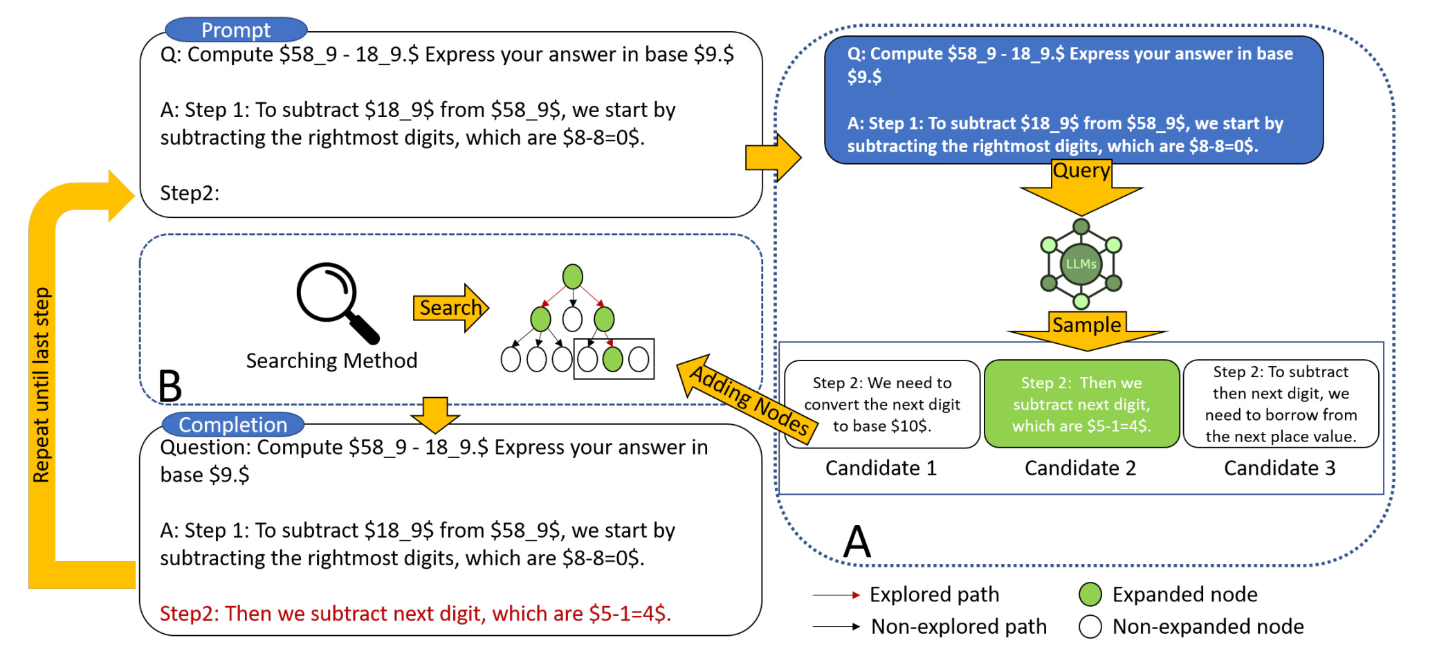
Example: The 24 Game

Consider the classic 24 Game: you're given a set of numbers, and the challenge is to apply arithmetic operations to reach the target number 24. The task requires reasoning and deciding which operations to apply, in what order, and how intermediate steps interact.

1. Thought corresponds to one or more steps of applying operations to the input numbers 4,9,10,13. For example, use + for the first two numbers: 4+9=13, resulting in 10,13,13 left.

2. Generate several “thoughts“ using the Propose Prompt (see Figure below, box (a)). This results in several thought candidates: e.g., 4+9=13 or 10-4=6

3. Evaluate the candidate by prompting another LLM with Value Prompt (see Figure below, box (b)). The LLM will decide whether it is possible to continue the thought

4. Do the tree search based on LLM evaluations with the node as the candidate thought. If LLMs say it is impossible to continue. In this case, “4+9=13” node is impossible to continue, so the search algorithm will not go further. Instead, it chooses “10-4=6” to continue the generation and search process.

From this example, we can construct a general framework for test-time scaling of LLMs as follows:

A general framework for test-time scaling. Source: [5]

There are 3 main components of the framework:

• Verification: Evaluate the quality or correctness of generated outputs.

• Generation / Search: Produces reasoning candidates through sampling or exploration.

• Improvement with Feedback: Refines the model or outputs using signals from verification or external supervision.

As we shall see, the most recent methods aim to enhance one or more of these components. The last one will be discussed in my next blog. Now, let’s explore the first component in the next section.

---

Process Reward Models: Defining What’s "Good Reasoning"

For many reasoning-intensive tasks, such as math word problems, code generation, or symbolic logic, the final answer is verifiable. That is, given a question and a proposed solution, we can automatically check whether the answer is correct. This verifiability makes it possible to supervise models during training by rewarding correct outputs, even if we don't label every intermediate step.

However, this introduces a subtle challenge: not all paths to the correct answer are equally good. A model might stumble into the right solution by chance, through memorization, or via logically inconsistent steps. If we only reward the final answer, we risk reinforcing spurious or incoherent reasoning.

This realization has spurred interest in Process Reward Models (PRMs), which aim to evaluate and guide the reasoning trajectories of LLMs, rather than just their final outputs.

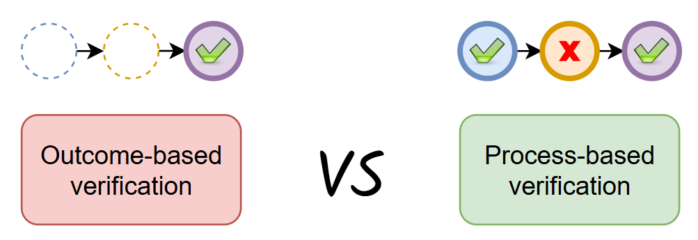
From Outcome-Based to Process-Based Evaluation

Traditional reinforcement learning approaches often focus on outcome-based rewards, evaluating the correctness of the final answer. However, this method overlooks the variety of the reasoning path taken to arrive at that answer. PRMs address this gap by assigning rewards to intermediate reasoning steps, promoting coherent and logical progression throughout the problem-solving process.

While verifying a final answer can often be automated (e.g., is the math answer correct?), supervising the reasoning process itself is a much harder problem. There’s no straightforward way to automatically label whether an intermediate step is valid or logically sound. An early paper named 👉“Let’s Verify Step by Step” tackles this head-on by manually labeling the reasoning process using human annotators [6]. The researchers asked labelers to evaluate the correctness of each step in the solution paths generated by LLMs.

Manual labeling of the reasoning step quality. Source: [6]

This resulted in PRM800K, which contains 800K step-level labels, annotated across 75K model-generated solutions spanning 12K problems. Each step is labeled for correctness, enabling fine-grained reward modeling for reasoning.

The researchers then aim to train reward models in two regimes:

• Large-scale: They use the labeled dataset to fine-tune GPT-4, aiming to build high-quality outcome and process reward models (ORMs and PRMs). While this setup pushed performance to the state-of-the-art, differences in training data made direct comparisons between ORMs and PRMs tricky.

• Small-scale: To isolate the effect of supervision and enable controlled ablations, they trained smaller models from scratch. This allows using large models to create labeled data for training small models. This setup allowed them to probe how process supervision affects reasoning quality under more constrained conditions.

Here, the paper focuses on training reliable reward models rather than running a full RL loop. They evaluate the reward models by using the best-of-N approach:

1. Generate N candidate solutions for each problem.

2. Use the reward model for assigning scores to the solutions to rank them.

👀 For PRM, when determining a solution-level score, they either use the minimum or the product of step-level scores as a reduction.

3. Pick the top-ranked one.

4. Check if the final answer is correct.

The evaluation metric is the fraction of problems where the top-ranked solution is correct. The results reveal that PRM can detect the wrong steps in reasoning solutions. Compared to other methods, such as ORM or Majority Voting, PRM scales much better as N increases:

❌ One major bottleneck for training PRMs is the need for high-quality, step-level annotations, especially in domains like math, where reasoning is complex and annotators need domain expertise.

❌ Human labeling at this level of granularity is expensive and time-consuming, making it difficult to scale PRM training for practical use.

Therefore, recent papers propose an automatic process supervision framework to reduce reliance on manual labeling. For example, in the 👉MATH-SHEPHERD paper [7], the researchers define a step's quality by how likely it is to lead to the correct final answer. Intuitively, here's how it works:

• Start with a math problem and its ground-truth final answer.

• From an intermediate step in a candidate solution, decode multiple possible future reasoning paths using a fine-tuned LLM.

• Check how often these paths arrive at the correct final answer.

• The more reliably a step leads to correct answers, the higher its correctness score.

Automatically assigning rewards to the reasoning steps. Source: [7]

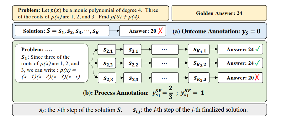
In particular, given a reasoning step s_i​, they generate a set of N completions (i.e., possible continuations of reasoning) using a fine-tuned LLM:

\( \left\{ (s_{i+1,j}, \dots, s_{K_j,j}, a_j) \right\}_{j=1}^{N} \)

where a_j​ is the final answer reached in the j-th continuation. The set of all decoded answers is:

\(A = \{ a_j \}_{j=1}^N \)

To score the quality y_si​​ of step s_i​, we consider two estimation strategies:

• Hard Estimation (HE): A step is labeled as "good" (reward =1) if any of its completions reaches the correct answer a∗:

\(y_{s_i}^{\text{HE}} = \begin{cases} 1 & \text{if } \exists a_j \in A \text{ such that } a_j = a^* \\ 0 & \text{otherwise} \end{cases}\)

• Soft Estimation (SE): Calculate the step-reward score as the frequency with which the completions arrive at the correct answer:

\(y_{s_i}^{\text{SE}} = \frac{1}{N} \sum_{j=1}^{N} \mathbb{I}(a_j = a^*) \)

How to Train a Process Reward Model (PRM)

Formally, a PRM maps a problem P and a reasoning step S to a (positive) reward R:

\(\text{PRM}: P \times S \rightarrow \mathbb{R}_{+} \)

The training objective treats step-level scoring as a binary classification problem. For a solution with K reasoning steps {s₁,s₂,…,s_K}, the PRM learns to assign scores r_si∈[0,1] indicating the quality of each step, i.e., >0.5 good, otherwise bad. The cross-entropy loss is applied over all steps:

\(\mathcal{L}_{\text{PRM}} = \sum_{i=1}^K y_{s_i} \log r_{s_i} + (1 - y_{s_i}) \log (1 - r_{s_i}) \)

where:

• y_si​​∈{0,1} is the target label indicating whether step s_i is good,

• r_si is the PRM's predicted score (typically after applying a sigmoid).

The training results show that Soft Estimation is better than Hard Estimation:

Once we’ve trained a PRM to score each reasoning step, we can take the minimum score across all steps in a solution as the ranking score in the best-of-N approach. The authors even go further by integrating self-consistency with reward models:

1. First, generate multiple candidate solutions with

2. Group these solutions by their predicted final answer.

3. Within each group, aggregate their PRM scores.

4. Finally, select the answer that is not just the most frequent, but the one supported by high reward scores.

Formally, the final answer chosen under this combined scoring strategy is:

\(a_{\text{sc+rm}} = \arg\max_{a} \sum_{i=1}^{N} \mathbb{I}(a_i = a) \cdot \text{PRM}(p, S_i) \)

More importantly, combining fine-tuning LLMs with the test-time strategy above (SHEPHERD) yields awe-inspiring results:

However, treating the PRM training task as a classification problem, i.e., labeling each step s_i as either "correct" or "incorrect", is not always perfect:

❌ It overlooks the structure of the trajectory, including the dependencies among steps, the cascading effect of earlier errors, and the varying importance of each step in solving the overall task.

❌ Each state is treated in isolation, leading to reward assignments that are often misaligned with the actual contribution of a step toward reaching a correct final answer.

To address this, a recent work introduces a new perspective: 👉Process Q-value Modeling (PQM) [8]. Instead of predicting correctness as a binary label, PQM frames the reasoning process as a Markov Decision Process (MDP) and aims to estimate the Q-value—that is, the expected probability that a particular action (a reasoning step) from a given state will lead to a correct final answer.

In this framework:

• The state s_h=(x,a_1:h−1) represents the prompt x and prior steps a_1:h−1.

• The action a_h is the generated reasoning at step h.

• The policy π(a_h∣s_h) represents the LLM.

• The Q-value Q(s_h, a_h) estimates how promising this step is in achieving the correct final answer.

Here, the Q-value implicitly defines a process reward: good steps raise the probability of success, and bad ones diminish it. This leads to a comparative training objective, where the PRM learns to rank better trajectories (or sub-trajectories) higher than weaker ones. Crucially, this also recovers classification-based PRMs as a special case when only terminal correctness is available and steps are independent.

The paper offers several theoretical results:

• The Q-value for a reasoning step can be defined as the inverse sigmoid of the probability that a trajectory leads to a correct final answer, under a given policy.

• Then, the Q-value represents the likelihood that a partial action sequence will result in a correct answer, making it a natural fit for evaluating intermediate reasoning steps.

• Under deterministic settings, the advantage function (a form of temporal differences of values) can be treated as a reward function due to potential-based reward shaping.

• Among correct steps, later ones have higher Q-values; among incorrect steps, later ones have lower Q-values.

• The Q-value of the first correct step is greater than that of the initial state, which is in turn greater than that of the first incorrect step.

• Final findings: Q-values of incorrect steps decrease over time, followed by the initial state's Q-value, then increasing Q-values of correct steps, establishing a clear separation between correct and incorrect reasoning trajectories.

A central goal in training PQM with rankings is not just to distinguish between correct and incorrect actions but to reflect the magnitude of the difference between them. While the classical Plackett-Luce (PL) model provides a way to capture ranking relationships, it falls short in our setting where Q-value gaps between correct and incorrect steps can be highly uneven and consequential. Therefore, the authors propose a Q-margin-based comparative loss that is sensitive to Q-value differences, capturing not only which step is better but also how much better.

Based on the theoretical findings above, the optimal Q-values induce a strict ordering:

\(Q^*_{w_{|W|}} < \cdots < Q^*_{w_2} < Q^*_{w_1} \ll Q^*_0 < Q^*_{c_1} < Q^*_{c_2} < \cdots < Q^*_{c_{|C|}} \)

where W and C denote the set of wrong and correct step indices, respectively. To enforce this structure during training, the authors define the loss:

\(\mathcal{L}_{\text{theorem}} = -\frac{1}{H} \left[ \sum_{t=2}^{|W|} \log \frac{\exp(Q_{w_t})}{\sum_{q=1}^{t} \exp(Q_{w_q})} + \sum_{t=0}^{|C|} \log \frac{\exp(Q_{c_t})}{\sum_{q=0}^{t} \exp(Q_{c_q}) + \sum_{w \in W} \exp(Q_w + \zeta)} \right]\)

Here, ζ is a margin hyperparameter that magnifies the penalty for incorrect steps by adding a positive bias to their exponentiated Q-values. Let’s explain the equation:

• The first term models the relative ranking among incorrect steps W. The PL-style ranking is used to penalize incorrect steps that receive higher Q-values than worse ones. Starting the sum at t=2 ensures we compare each step against all higher-ranked (i.e., better, smaller indices) incorrect steps. For example, if the model is estimating wrongly, like Q_w2>Q_w1, the loss is greater, and thus minimizing the loss helps.

• The second term compares correct steps C with all incorrect ones and “less correct“ steps. The margin ζ encourages a clear separation between correct and incorrect actions, not just in rank but in actual Q-value magnitude.

While the full loss L_theorem captures nuanced structure, it assumes accurate annotation of incorrect steps, which is rarely guaranteed in practice. Most datasets label all steps after the first mistake as "wrong," even if some are less severe. This motivates a simplified yet robust loss:

\(\mathcal{L} = -\frac{1}{|C|} \sum_{t=0}^{|C|} \log \frac{\exp(Q_{c_t})}{\sum_{q=0}^{t} \exp(Q_{c_q}) + \sum_{w \in W} \exp(Q_w + \zeta)} \)

This loss ignores the internal ranking among wrong steps (the first term in L_theorem) and concentrates on learning a clear separation margin between the correct and incorrect actions.

The paper demonstrates better performance than other PRM training losses, such as using binary classification’s cross-entropy or MSE loss:

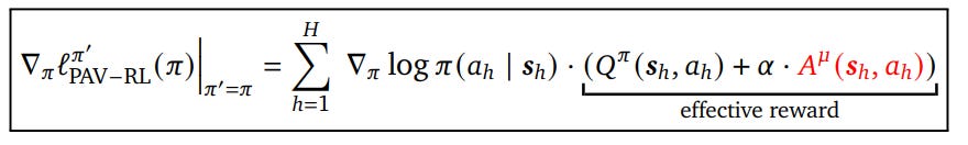
From a different perspective, researchers argue that intermediate, or process, rewards should act as fine-grained supervision, guiding the model at each step in a way that supports the long-term objective of arriving at the right outcome. This perspective differs from the conventional approach, which often assumes process rewards should strictly reflect the mathematical correctness or semantic relevance of each step. In contrast, large language models may need to take detours—generating seemingly trivial or redundant steps—to ultimately find a successful reasoning trajectory. Penalizing such steps too early or too harshly can prematurely collapse promising search paths. Therefore, the paper proposes focusing on rewarding the progress, which can be estimated by advantage functions rather than the Q-value [9]. They name the method 👉Process Advantage Verifiers (PAV).

To see why Q-value may not be an ideal estimation of progress, imagine we're running a beam search to explore different reasoning paths. Each path (or trace) is a sequence of steps, and we want to keep the most promising ones in the beam. A natural approach might be to retain those with the highest Q-values. But Q-values inherently entangle two things—the value of the action and the value of the state it came from. That creates a problem. If we compare actions from different states purely based on their absolute Q-values, we risk keeping steps that decrease our likelihood of success, simply because they come from "stronger" states:

Rather than looking at raw Q-values, we should focus on the change they induce—that is, the progress a step makes toward success. This is captured by the advantage function:

\(A_{\pi}(s_t, a_t) = Q_{\pi}(s_t, a_t) - V_{\pi}(s_t) = Q_{\pi}(s_t, a_t) - Q_{\pi}(s_{t-1}, a_{t-1}) \)

Advantage tells us whether a step improved or hurt our chances of solving the problem. A positive advantage means the step made meaningful progress; a negative one means it sets us back. By supervising the model with these advantage values, we reward real progress, not just proximity to good outcomes.

Furthermore, the advantage doesn’t need to be computed under the same policy that we’re training. As the paper argues, we may want to compute these progress signals under a stronger prover policy μ, different from our current base policy π. This prover acts like an expert verifier, assessing whether a step truly advances reasoning under its own more accurate value estimates.

The authors then propose components of the loss to train the policy:

• Outcome reward (of course) of the base policy:

• The advantage of the prover policy:

Using policy gradient methods, we can have the gradient to update the policy as:

Now, the remaining question is: 🧠 How Should We Choose the Prover Policy μ?

• Don’t set μ=π (base policy):

  • This reduces to standard outcome-based training.

  • The advantage A_π adds no extra supervision, especially harmful if π is weak, since both Q_π and A_π will be close to zero.

• Don’t use a very weak μ:

  • Just like a weak base policy, a weak prover produces flat or noisy advantage signals.

  • Beam search and training signals become unreliable.

• Don’t use an overly strong prover μ:

  • A strong prover can succeed regardless of trivial or irrelevant steps (e.g., restating the question).

  • As a result, Q_μ stays constant across such steps, leading to A_μ​≈0.

  • Training then rewards superficial behavior and fails to improve reasoning.

To prove the points, the author conducts a synthetic experiment (didactic setup):

• Goal: Train a policy π to generate a sequence that contains a hidden sub-sequence y∗ from a vocabulary V={1,2,…,15}.

• Reward: Sparse and terminal — the agent only receives a reward of 1 if y∗ appears in the output y; otherwise, 0.

• Prover policy μ: A procedural policy controlled by a scalar γ>0; as γ increases, μ becomes more effective, reaching perfect accuracy as γ→∞.

• Assumption: The setup uses Oracle access to true Q_π and A_μ​ to avoid approximation errors from learned models.

The results prove the point that A is better than Q, and middle γ is best.

The results on the MATH dataset confirm the points:

---

Search and Planning with RL

The second component of test-time scaling is the generation and search process. RL allows us to help LLMs actively explore the space of reasoning steps to discover new, high-reward trajectories. When paired with search, RL becomes a powerful tool, not just for improving final answers, but for shaping how the model thinks.

Imagine solving a math problem. You might try several intermediate calculations, discard a few, refine your strategy, and finally reach a solution. This iterative process of proposing, testing, and revising steps is precisely what we want LLMs to emulate. Pure next-token prediction is too myopic for this, while search gives the model the "lookahead" it needs.

TTC Scaling Using Classic Search Algorithms

Early approaches, such as ToT [4], involve using straightforward brute-force search algorithms, such as Breadth-First Search (BFS) and Depth-First Search (DFS). For example, a simple search framework will look like this

• Step Sampling: At each step, use the question and prior reasoning to sample B next steps via an LLM.

• Reasoning Tree:

  • Organize reasoning as a tree:

    • Root: question

    • Node: current generated text

    • Edge: reasoning step

    • Leaf: final answer

  • A search algorithm selects a node to expand.

• Expansion: Add the selected node's step to the prompt and sample new steps.

• Stopping: Halt when an answer is found or a step/computation limit is reached.

Search in action. Source: [10].

The key here is the search algorithm. 👉MindStar (M*) [10] proposes an LLM-inference-time search procedure using Levin Tree Search, which is a best-first tree search algorithm. This kind of search avoids trying to select all nodes to expand. Thus, a criterion should be employed to choose which node or reasoning step to select. Here, the authors assess each reasoning step with the aforementioned PRM.

Formally, given a current node n_d​ and a candidate's next step e_d​, the PRM outputs a reward:

\(P(n_d, e_d) = r_d \in [0, 1] \)

A high r_d​ means the step is likely valid and consistent with prior reasoning. Once we score the child nodes with PRM, we must decide which node to expand next. Two strategies are examined:

• Beam search selects the (top) next steps with the highest rewards:

  \(e^*_d = \arg\max_{e_i \in \{e^1_d, \dots, e^N_d\}} P(n_d, e_i) n_{d+1} = [n_d \oplus e^*_d]\)

• Levin Tree Search (LevinTS): LevinTS improves on beam search by balancing cost and probability:

  • Cost: the cost of the path (the smaller the better)

  • Probability: reflects how likely a node leads to a solution (the higher the better)

The paper proposes the cost function as:

\(f(n) = e^{\tau \cdot i_{tok}} \)

where:

• i_tok = number of tokens in n

• τ = temperature (controls search aggressiveness)

And the probability π(n) is recursively defined as:

\(\pi(n) := \pi(n') \cdot \frac{e^{P(n', e')}}{\sum_{i=1}^{N} e^{P(n', e_i)}} \)

where n has parent n′ connected by an edge e′.

LevinTS expands nodes in order of increasing f(n)/π(n), offering a guaranteed token budget:

\(|\bar{N}(\text{LevinTS}, N_g)| \leq \min_{n \in N_g} \frac{f(n)}{\pi(n)} \)

where N_g is a set of target nodes.

We can see these search algorithms improve LLMs significantly:

Sometimes, reasoning involves complicated planning, and to test LLM reasoning, we can use planning benchmarks such as maze navigation. Inspired by this, 👉LLM-A* paper aims to evaluate and improve LLMs on path planning [11].

Example of a path-finding problem. Source: [11].

The gist of LLM-A*: a hybrid algorithm that combines the optimality of A* with the high-level reasoning capabilities of an LLM. Together with A*, the LLM acts as a planning guide, suggesting waypoints (intermediate targets) based on its understanding of the start, goal, and obstacles.

• The algorithm begins like A*: define the start and goal, initialize the OPEN = {s₀} and CLOSED ={∅} lists, and use a cost function f(s) = g(s) + h(s). Here, A* employs a heuristic function h(s) to estimate the cost from a node s to the goal, and a cost function g(s) to track the exact cost from the start to s.

• But before the search begins, the LLM is prompted with the environment information and asked to generate a target list T: a series of waypoints that form a plausible path to the goal.

• As A* proceeds, it modifies its f(s) score to bias toward the current LLM-suggested waypoint t:

\(f(s) = g(s) + h(s) + cost(t, s) \)

👀 The cost(t,s) term encourages A* to prioritze solutions that contain LLMs’ waypoints.

• Once the current target t is reached, it updates to the next in the sequence, continuously steering the local search using global LLM knowledge.

• Crucially, the algorithm also verifies that all waypoints in T are outside obstacle zones and contain the correct start and goal nodes, correcting any LLM hallucination.

LM-A* uses several prompting techniques to extract better target paths from the language model:

• Few-Shot Learning: Demonstrates the LLM 5 by showing 5 demo examples of correct paths before prompting for a new one, thereby increasing reliability without requiring training.

• Chain-of-Thought (CoT): Encourages the LLM to reason step-by-step rather than jumping to the answer. This is particularly helpful in more complex environments where multi-step logic is essential.

• Recursive Path Evaluation (RePE): Breaks the planning into three LLM-driven stages:

  1. Analyze the environment,

  2. Generate a step,

  3. Evaluate that step.

  This recursion mimics approaches like ReAct and Self-Reflection but focuses entirely on internal reasoning, without environmental feedback.

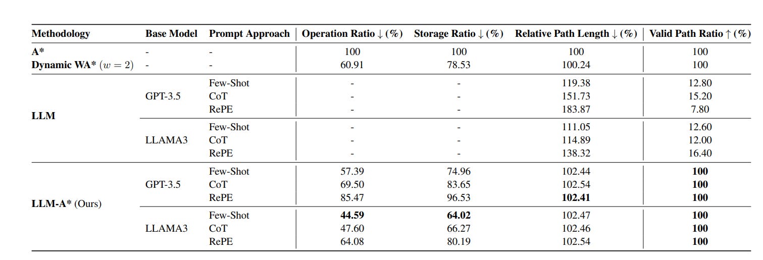
Finally, the results demonstrate that LLM-A* outperforms LLM alone significantly in the benchmark.

❌ One big issue with relying on classic search algorithms is the choice and design of the cost function f(). Prior approaches often hinge on carefully engineered utility functions (e.g., number of tokens for text and distance for path planning), which introduce practical limitations.

An elegant alternative is to frame multi-step reasoning as an MDP. Here, each reasoning trajectory maps to a path through a decision space, where the state is the input prompt plus previous steps, the action is the next proposed token, and the Q-value can be used as the cost function. The paper 👉Q* leverages this structure by adopting a best-first decoding strategy, inspired by A* search [12].

👀 A bit different from the aforementioned papers like PQM that model action as a reasoning step consisting of multiple tokens, the action in Q* is single token.

Q* framework. Source: [12]

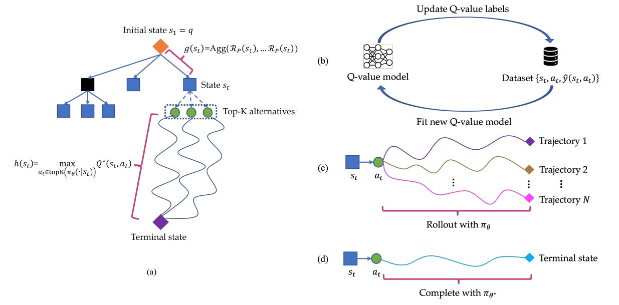
Specifically, Q* casts reasoning as a heuristic search problem. Each partial reasoning path s_t​ is scored using an A*-style utility function:

\(f(s_t) = g(s_t) + \lambda h(s_t) \)

• g(s_t​): Aggregated reward along the path so far.

• h(s_t): Heuristic estimate of the utility-to-go.

• λ: A scalar balancing the two terms.

To compute g(s_t), Q* uses an aggregation function of a reward function R_P​ that reflects task-specific preferences (e.g., correctness, coherence, confidence):

\(g(s_t) = \text{Agg}(R_P(s_1), \ldots, R_P(s_t)) \)

For the heuristic h(s_t), Q* uses the optimal Q-value:

\(f(s_t) = g(s_t) + \lambda \max_{a_t \in \text{top-}K(\pi_\theta(\cdot|s_t))} Q^*(s_t, a_t) \)

Rather than exploring all possible continuations, Q* limits candidates to the top-K tokens proposed by the LLM.

The key challenge is estimating the optimal Q-value Q*(s_t,a_t) for a frozen LLM policy π_θ. To do this, Q* learns a proxy Q-value function Q̂ from offline trajectories:

\(\hat{Q} = \arg\min_Q \frac{1}{NMT} \sum_{i=1}^{N} \sum_{j=1}^{M} \sum_{a_t \in a_{ij}} (Q(s_t, a_t) - \hat{y}(s_t, a_t))^2 \)

where M is the number of actions in a trajectory and N is the number of trajectories. ŷ​(s_t​,a_t​) is a label approximating the true Q-value, computed using the following strategies:

1. Using Fitted Q-Iteration, labels are constructed recursively:

\(\hat{y}^\ell(s_t, a_t) = \begin{cases} R(s_t, a_t) & \text{if } t = T \\ R(s_t, a_t) + \gamma \max_{a_{t+1} \in \text{top-}K} \hat{Q}^{\ell-1}(s_{t+1}, a_{t+1}) & \text{otherwise} \end{cases}\)

This process alternates between updating labels and training Q̂ for L iterations.

2. Learning from Rollouts: run random or MCTS rollouts from (s_t,a_t) and assign labels based on the best future trajectory:

\(\hat{y}(s_t, a_t) = R(s_t, a_t) + \max_{\tau \sim \mathcal{P}} \sum_{t' = t+1}^{T} \gamma^{T - t'} R(s'_{t'}, a'_{t'}) \)

3. Using a Stronger LLM: if a stronger LLM π_θ*​ is available (e.g., GPT-4), complete the reasoning with it to estimate the future reward:

\(\hat{y}(s_t, a_t) = R(s_t, a_t) + \sum_{t' = t+1}^{T} \gamma^{T - t'} R(s^*_{t'}, a^*_{t'}) \)

where:

\(s_{t'}^* = [s_t; a_t; a_{t+1}^*; \ldots; a_{t'-1}^*] \)

\(a_{t'}^* \sim \pi_{\theta^*}(\cdot \mid s_{t'}^*) \)

❌ While classic search-inspired frameworks like A* provide structured guidance for stepwise reasoning, they often rely on static heuristics and limited lookahead.

Beyond Search with Planning

To explore deeper decision spaces and balance exploration with exploitation, recent approaches turn to Monte Carlo Tree Search (MCTS)—a planning algorithm that enables LLMs to simulate multiple reasoning trajectories and refine their outputs through iterative rollouts. This shift empowers LLMs to deliberate more thoroughly, especially on complex tasks with long-horizon dependencies.

Although classical MCTS depends on access to an explicit environment model to simulate forward trajectories, this assumption is often unnecessary in language-based tasks. A key insight exploited by 👉Language Agent Tree Search (LATS) [13] is that for most language model (LM) environments—such as web navigation, multi-step reasoning, or tool use—we can reconstruct any prior state simply by restoring the full-text history. This removes one of the main barriers to applying MCTS in natural language settings and opens the door to powerful planning capabilities within LMs.

LATS adapts MCTS to language agents by interpreting each node in the tree as a structured tuple:

\(s = [x, a_{1:i}, o_{1:i}]\)

where x is the original task input, a_1:i is the action sequence taken so far (including reasoning traces), and o_1:i are the corresponding observations or feedback. The search tree is built incrementally using six operations:

1. Selection: Starting from the root, LATS uses the UCT criterion to traverse down the tree until it reaches a leaf node.

\(\text{UCT}(s) = V(s) + w \sqrt{\frac{\ln N(p)}{N(s)}} \)

• V(s) is the estimated value of node s

• N(s) is the number of visits to node s

• N(p) is the number of visits to s's parent p

• w is the exploration weight

2. Expansion: At the selected node, the LM samples n next-step actions:

\(a_t^{(1)}, \ldots, a_t^{(n)} \sim p_\theta(\cdot|s)\)

3. Evaluation: Each new node is scored with a novel value function:

\(V(s) = \lambda \cdot \text{LM}(s) + (1 - \lambda) \cdot \text{SC}(s) \)

• LM(s) is a scalar score predicted by the language model, prompted to end its reasoning trace with a self-assessed rating,

• SC(s) is a self-consistency score, aggregating agreement across multiple LM samples from the same node.

4. Simulation: LATS recursively samples and simulates actions from the current node until a terminal state is reached. The LM executes this by generating the remainder of the trajectory.

5. Backpropagation: Upon reaching a terminal state and obtaining a reward r, LATS updates all ancestor nodes along the path s₀​→s₁​→⋯→s_ℓ:

\(V(s_i) = \frac{V(s_i) \cdot (N(s_i) - 1) + r}{N(s_i)} \)

Here, the visitation count is updated as:

\(N(s_i) \leftarrow N(s_i) + 1,\)

6. Reflection: When a trajectory fails, the LM is prompted to reflect on its reasoning and generate a natural language critique. This is stored and injected as additional in-context information in future rollouts, providing “semantic gradient” signals that improve decision-making without explicit gradient descent. The prompt for reflection is like this:

You are an advanced reasoning agent that can improve based on self-reflection. You will be given a previous reasoning trial in which you were given access to a shopping website and a specific type of item to buy. You were given access to relevant context and an item to …

MCTS in LATS. Source: [13].

As the results speak, LATS improves on tasks that require reasoning and tool use (internet search):

As we’ve seen, many recent papers propose integrating search and planning with RL concepts to improve LLM reasoning, ranging from beam search guided by reward models to complex tree-based planning algorithms. However, this raises an important question: 🧠 Is more complexity always better?

A recent empirical study titled 👉Scaling LLM Test-Time Compute Optimally Can Be More Effective Than Scaling Model Parameters performed comprehensive evaluations that revealed many insights [14].

Core Idea: Test-Time Compute as a Resource:

• Instead of scaling parameters, we scale how we use compute at test time (e.g., number of samples, depth of revisions, search strategy).

• Given a prompt and a fixed compute budget N, different compute strategies yield different accuracies.

• Some questions benefit more from refinement (e.g., iterative revisions), while others require broader exploration (e.g., sampling diverse solutions in parallel).

Formally, we define Target(θ, N, q) as the output distribution, given a strategy θ, budget N, and prompt q.

• The goal is to find the optimal search strategy:

\(\theta^*_{q, y^*(q)}(N) = \arg\max_\theta \mathbb{E}_{y \sim \text{Target}(\theta, N, q)}[\mathbf{1}_{y = y^*(q)}] \)

There are two main components in strategy:

1. Proposal Distribution: how candidate answers are generated (e.g., revision vs. independent sampling).

2. Verifier: how candidates are judged (e.g., majority vote, best-of-N, or scoring models like ORMs or PRMs).

The paper studies several options for strategies:

Common searching stragties. Lookahead search may include A* and MCTS. Source: [14].

👀 The intuition is that, for easy problems, simple search may suffice, yet for hard problems, it is better to sample diverse reasoning paths up front.

This requires approximating question difficulty to guide how computing should be allocated. 🧠 How to estimate problem difficulty?

• Two ways:

  • Oracle difficulty: uses ground-truth labels (ideal but impractical).

  • Model-predicted difficulty: uses verifier scores to estimate difficulty without access to answers.

We often assume more sophisticated search equals better performance. But the empirical results say: not always. In particular,

• Beam search wins early: At low-generation budgets, beam search significantly outperforms best-of-N. But this advantage vanishes as the budget increases.

• Lookahead search underperforms: Despite being more powerful, it performs worse due to:

  • Costly rollouts.

  • Over-optimization of the verifier (PRM), leading to repetitive or trivial outputs.

• Diminishing returns from search are real: As shown in some failure cases, stronger search just amplifies bad verifier signals, generating:

  • Repetitive steps.

  • Overly short or spurious solutions.

Using difficulty-conditioned compute allocation—i.e., scaling search per question difficulty—improves efficiency:

• With oracle difficulty bins, the compute-optimal strategy nearly matches the best-of-64 using only 16 generations.

• Even with model-predicted bins, the gains largely hold.

Last but not least, the paper also explores improving the model’s proposal distribution by teaching it to revise its answers. This technique can be combined with parallel search approaches like best-of-N:

Sequential revision approaches. Source: [14].

Unlike naive self-correction (which often fails), fine-tuning a model to iteratively refine previous answers yields clear improvements. So, they do supervised fine-tuning (SFT) on trajectories composed of a sequence of incorrect answers followed by a correct one. This trains the model to identify and correct mistakes in context rather than discard prior attempts and restart.

At inference time, the finetuned model generates sequential revisions, each conditioned on the latest few attempts (up to four). Empirically, performance improves with each revision step, showing the model effectively learns to self-correct over time.

Key insights: They find a tradeoff between sequential revisions and parallel sampling at test time. The optimal ratio depends on both the compute budget and the question’s difficulty:

• Easier questions perform best with purely sequential computation.

• Harder questions benefit from a balanced mix.

By adjusting this ratio per question, they can outperform standard best-of-N baselines using up to 4× less compute.

If you realize, all of these papers assume that the search process will eventually lead to a correct answer. In other words, they assume that LLMs already know the right answer, but just need the right trigger to reach it.

This is exactly the hypothesis behind 👉AlphaMath:

👀 Pre-trained LLMs already contain rich mathematical knowledge. The challenge is not learning from scratch, but activating this latent reasoning through better prompts and smarter search.

The paper follows prior works in modeling text generation as an MDP, where the LLM acts as a policy: At step t, state = partial solution s_t, action = next step a_t, and
the transition is deterministic:

\(s_{t+1} = \text{Cat}(s_t, a_t), \quad \pi_\theta(a_t \mid s_t) = \text{LLM}(a_t \mid s_t) \)

Here, to find the optimal reasoning path, AlphaMath combines:

• A Monte Carlo Tree Search (MCTS) to balance exploration and exploitation, which is typical as in prior work:

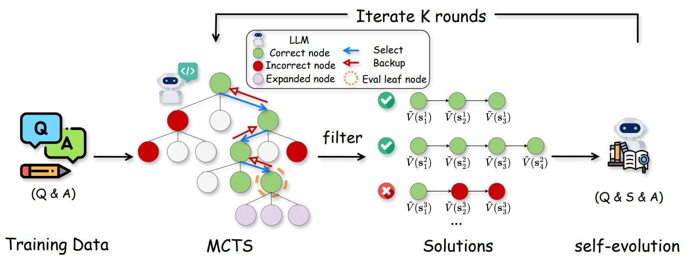
• The novel bit is that a lightweight value model was added to the same LLM to judge intermediate reasoning quality

Not relying on the value estimated in MCTS, the paper proposes a value model V_ϕ(s) to estimate how likely a partial solution will lead to a correct final answer.

👀 A value model can generalize to new states, which will be useful to boostrap the value estimation of MCTS.

Training this model relies on Monte Carlo evaluation from multiple rollouts:

\(V_e(s_t) = \frac{1}{N} \sum_{i=1}^{N} r(a^{(i)}_{\geq t}, s^{(i)}_{> t} \mid s_t) \)

Then, we can optimize the value model via regression:

\(\mathcal{L}_{V_\phi}(s) = \left(V_\phi(s) - V_e(s)\right)^2 \)

Given the value model, the MCTS phase uses both policy and value models to guide simulations:

Summary of 4 MCTS steps in AlphaMath. Source:[15].

Here, some steps introduce novelty. First, action selection uses a PUCT-style rule:

\(a_t = \arg\max_a \left[ \hat{Q}(s_t, a) + c_{\text{puct}} \cdot \pi_\theta(a \mid s_t) \cdot \frac{\sqrt{N_{\text{parent}(a)}}}{1 + N(s_t, a)} \right] \)

Each term here has a clear role:

• Q̂ : This is the MCTS’s average return (value) obtained when taking action a_t at state s_t​, based on past simulations. It encourages picking the best-known option so far (exploitation).

• π_θ​(a∣s_t​): the likelihood of taking action a according to the current policy. It helps bias the search toward actions the model thinks are promising — this is a key LLM-specific addition. It helps reduce the number of required simulations by starting from smart guesses (prior guidance).

• The counting term favors actions that haven’t been visited much.

  • If N(s_t,a)is low, the denominator is small, so the whole term becomes large → we explore new actions.

  • As N(s_t,a) increases (more visits), the term shrinks, reducing exploration pressure.

Second, the evaluation step is a mix of reward observation and value model estimation:

\(\hat{V}(s_t)^{(i)} = (1 - \lambda) \cdot V_\phi(s_t) + \lambda \cdot r\left( a^{(i)}_{t' \geq t},\, s^{(i)}_{t' > t} \mid s_t \right) \)

where i represents the i-th simulation. Given the current value estimation, we can do the backpropagation step to update the state-action value as:

\(\begin{align} N(s, a) &\leftarrow N(s, a) + 1 \\ \hat{Q}(s, a) &\leftarrow \frac{1}{N(s, a)} \sum_{j=1}^{i} \mathbb{I}_{s, a \rightarrow s_t} \, \hat{V}(s_t^{(j)}) \end{align}\)

After running N simulations with MCTS, we get a search tree with state-action values Q(s, a) stored at each node. Since the transition is deterministic, we assume for non-terminal nodes:

\(Q(s_t, a_t) = r(s_t, a_t) + V(s_{t+1}) = V(s_{t+1}) \)

This implies that we can estimate the MCTS’s value as:

\(\tilde{V}(s_{t+1}) = \hat{Q}(s_t, a_t) \)

This “ground-truth“ value will be used to train the value model.

Finally, although MCTS works, it’s slow. During deployment inference, to speed up inference, AlphaMath introduces Step-level Beam Search (SBS):

• At each step, generate B₂​ next-step candidates with the LLM

• Evaluate each with V_ϕ, keep top B_1​

👀 No simulation, no tree—just fast reasoning with value guidance. MCTS is just the tool for training the value model. When B₁=1, SBS becomes a fast MCTS approximation for real-time use.

The results show that SBS is much faster while keeping competitive performance:

---

Conclusion & What’s Next

This blog covered test-time reinforcement learning methods that guide large language models without further gradient updates. By treating reasoning as a sequential decision process, we leveraged techniques like:

• Classic Tree Search

• Monte Carlo Tree Search

• Process Reward Modeling

But even with advanced test-time methods like MCTS and beam search, the model’s reasoning remains externally guided and self-supervised by final answers only. These methods help with step selection, but they don’t change the model’s internal reasoning ability. 🧠 So what if we want to go further? What if we aim to improve the LLM’s internal reasoning competence, not just steer it at test time?

To do that, we need more than search—we need to update the model’s weights. This is where reinforcement learning during post-training comes in: by assigning reward signals not only to the final answer, but also to the quality and structure of intermediate reasoning steps, we can directly fine-tune LLMs to reason better from the inside out.

🔜 Next up: We'll study how reinforcement learning frameworks can be adapted to fine-tune LLMs for better reasoning, using novel rewards and RL algorithms, and more. Stay tuned. Reasoning is just getting smarter. 🧩🚀

---

References

[1] Achiam, Josh, et al. "Gpt-4 technical report." arXiv preprint arXiv:2303.08774 (2023).

[2] Jaech, Aaron, Adam Kalai, Adam Lerer, Adam Richardson, Ahmed El-Kishky, Aiden Low, Alec Helyar et al. "Openai o1 system card." arXiv preprint arXiv:2412.16720 (2024).

[3] Ji, Yixin, Juntao Li, Hai Ye, Kaixin Wu, Jia Xu, Linjian Mo, and Min Zhang. "Test-time Computing: from System-1 Thinking to System-2 Thinking." arXiv preprint arXiv:2501.02497 (2025).

[4] Yao, Shunyu, Dian Yu, Jeffrey Zhao, Izhak Shafran, Tom Griffiths, Yuan Cao, and Karthik Narasimhan. "Tree of thoughts: Deliberate problem solving with large language models." Advances in Neural Information Processing Systems 36 (2024).

[5] Kambhampati, Subbarao, Kaya Stechly, and Karthik Valmeekam. "(How) Do reasoning models reason?" Annals of the New York Academy of Sciences (2025).

[6] Lightman, Hunter, Vineet Kosaraju, Yuri Burda, Harrison Edwards, Bowen Baker, Teddy Lee, Jan Leike, John Schulman, Ilya Sutskever, and Karl Cobbe. "Let's verify step by step." In The Twelfth International Conference on Learning Representations. 2023.

[7] Wang, Peiyi, Lei Li, Zhihong Shao, Runxin Xu, Damai Dai, Yifei Li, Deli Chen, Yu Wu, and Zhifang Sui. "Math-Shepherd: Verify and Reinforce LLMs Step-by-step without Human Annotations." In Proceedings of the 62nd Annual Meeting of the Association for Computational Linguistics (Volume 1: Long Papers), pp. 9426-9439. 2024.

[8] Li, Wendi, and Yixuan Li. "Process reward model with q-value rankings." In The Thirteenth International Conference on Learning Representations, 2025.

[9] Setlur, Amrith, Chirag Nagpal, Adam Fisch, Xinyang Geng, Jacob Eisenstein, Rishabh Agarwal, Alekh Agarwal, Jonathan Berant, and Aviral Kumar. "Rewarding Progress: Scaling Automated Process Verifiers for LLM Reasoning." In The Thirteenth International Conference on Learning Representations. 2025.

[10] Kang, Jikun, Xin Zhe Li, Xi Chen, Amirreza Kazemi, Qianyi Sun, Boxing Chen, Dong Li et al. "Mindstar: Enhancing math reasoning in pre-trained llms at inference time." arXiv preprint arXiv:2405.16265 (2024).

[11] Meng, Silin, Yiwei Wang, Cheng-Fu Yang, Nanyun Peng, and Kai-Wei Chang. "LLM-A*: Large Language Model Enhanced Incremental Heuristic Search on Path Planning." In Findings of the Association for Computational Linguistics: EMNLP 2024, pp. 1087-1102. 2024.

[12] Wang, Chaojie, Yanchen Deng, Zhiyi Lyu, Liang Zeng, Jujie He, Shuicheng Yan, and Bo An. "Q*: Improving multi-step reasoning for llms with deliberative planning." arXiv preprint arXiv:2406.14283 (2024).

[13] Zhou, Andy, Kai Yan, Michal Shlapentokh-Rothman, Haohan Wang, and Yu-Xiong Wang. "Language agent tree search unifies reasoning, acting, and planning in language models." In Proceedings of the 41st International Conference on Machine Learning, pp. 62138-62160. 2024.

[14] Snell, Charlie, Jaehoon Lee, Kelvin Xu, and Aviral Kumar. "Scaling llm test-time compute optimally can be more effective than scaling model parameters." arXiv preprint arXiv:2408.03314 (2024).

[15] Chen, Guoxin, Minpeng Liao, Chengxi Li, and Kai Fan. "AlphaMath Almost Zero: Process Supervision without Process." In The Thirty-eighth Annual Conference on Neural Information Processing Systems, 2024.