
Improving LLM Reasoning with RL Post-Training
Surveying New Frontiers in Reinforcement Learning for Language Models (Part 3)

Large language models are getting better at reasoning, not because we made them bigger, but because we finally learned how to teach them after pre-training,a.k.a., post-training. Continuing our series on RL for LLM reasoning, today’s blog reviews recent papers that boost LLM reasoning capability via post-training with RL. If you care about strengthening a model’s intrinsic reasoning capabilities rather than bolting on expensive test-time scaling or multi-sample decoding, this overview highlights the methods that genuinely transform the model.

Table of Contents
Introduction
Reasoning remains one of the few capabilities where LLMs still fall short. When the conversation turns to boosting reasoning in LLMs, the default reaction is to immediately reach for test-time tricks: self-consistency, searching, multi-step decoding, or heavy ensembles. These methods are undeniably useful, but they all share a fundamental limitation: they are external scaffolds layered on top of an unchanged model.
Why RL Post-Training Matters for Reasoning?
Reasoning is ultimately about shaping the model’s internal search process, including how it attends, decomposes, checks, and revises its predictions. Supervised finetuning alone gives you patterns but rarely instills the principles needed for multi-step, error-sensitive reasoning. RL provides a way to push the model to explore diverse behaviors until it figures out the principles of reasoning on its own. When done right, the model starts solving tasks cleanly without huge decode budgets.
Over time, the model learns to prioritize reasoning strategies that generalize across tasks, rather than memorizing superficial patterns from the training data. This is why even relatively small models can outperform larger counterparts on multi-step reasoning benchmarks: the improvement comes from better internal reasoning processes, not from bigger parameter counts or expensive test-time tricks.
From Test-Time to Post-Training: What’s the Shift?
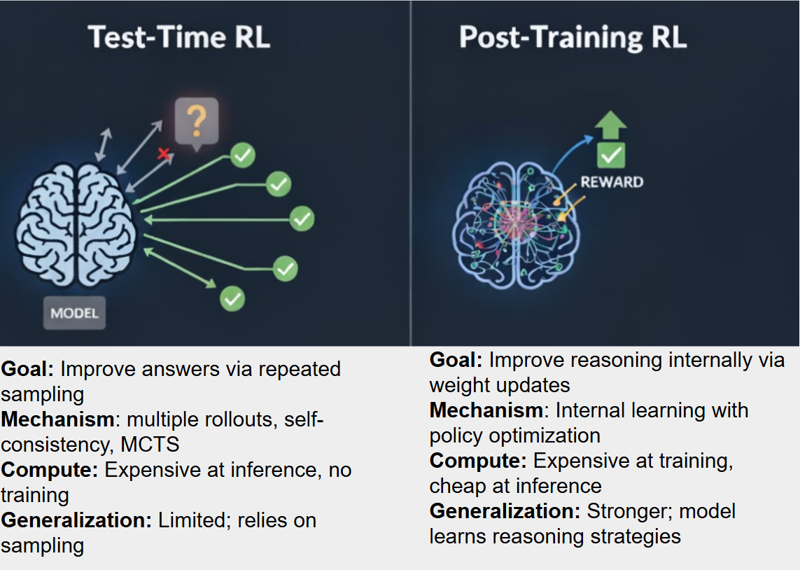
Test-time approaches rely on external scaffolds, generating multiple trajectories, performing searching and voting on the best answer, or sampling repeatedly to increase reliability. The model itself doesn’t change, so inference is expensive, and reasoning traces remain fragile depending on the samples.
Post-training RL takes a fundamentally different approach. By using reward-driven model updates, it reshapes the model’s internal heuristics, allowing it to plan, check, and revise its own reasoning based on the training rewards. As summarized in the figure below, post-training RL trades upfront training cost for cheaper, more reliable inference, cleaner reasoning traces, and stronger generalization. This shift marks the difference between forcing a model to reason through brute-force search and actually teaching it to reason internally.
It’s also important to understand how post-training RL differs from the other two major forms of post-training: supervised fine-tuning (SFT) and preference training.
SFT teaches the model to imitate reasoning patterns, but it requires ground-truth reasoning traces and can only learn what’s shown in the ground-truth data. There’s no pressure to explore, self-correct, or discover better reasoning paths. Preference training (like DPO or MRPO) adds a ranking signal, nudging the model toward preferred outputs, but it still operates passively: the model isn’t encouraged to search, plan, or discover new strategies, only to reshape its distribution around examples humans liked.
RL is different. RL gives the model room to experiment, take multi-step trajectories, encounter failure, and adjust its internal heuristics based on cumulative reward. That exploration loop is exactly what makes reasoning skills intrinsic rather than decorative. Put simply:
❌ Test-time scaling searches for the best outputs
❌ SFT teaches outputs
❌ Preference training teaches preferences over outputs
✔️ RL teaches the process that produces those outputs
And that’s why post-training RL is emerging as the most reliable way to move beyond surface-level reasoning gains. It turns reasoning from something we approximate at inference into something the model genuinely knows how to do. With that foundation in place, we can now study representative works on RL post-training, also called Reinforcement Finetuning (RFT).
DeepSeek-R1: The Tipping Point
DeepSeek began as an ambitious open-source initiative pushing the boundaries of efficient LLM training. Unlike many labs chasing scale at any cost, DeepSeek focused on pushing reasoning quality without gigantic models or massive inference budgets. That philosophy culminated in 👉DeepSeek-R1 [1], their breakthrough reasoning model.
R1 is built on a deceptively simple idea: outcome reward is all you need for RFT. It raises a research question:🧠 If a task has a verifiable final answer, can we train the model directly with policy gradients and a verifiable reward? For domains like math, logical inference, and structured problem solving, where correctness is binary, this setup is ideal. Instead of collecting huge preference datasets, relying on imitation or complicated process reward models, the model explores, fails, receives a clean reward, and gradually internalizes the principles of stepwise reasoning.
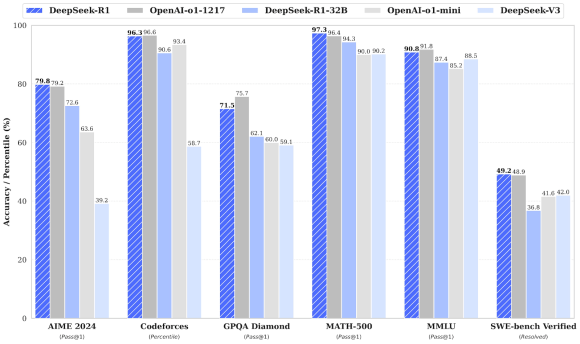
The DeepSeek team not only proved that this is doable, but they also open-sourced almost the entire training pipeline, showed how to make verifiable-reward RL work at scale, and did so at a shockingly low cost. Training was cheap, the resulting API was 27× cheaper than OpenAI’s reasoning models, and in many benchmarks, the performance was effectively equivalent.
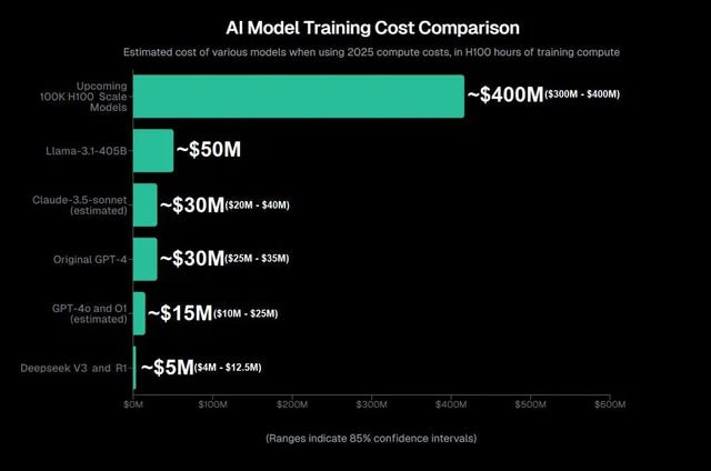
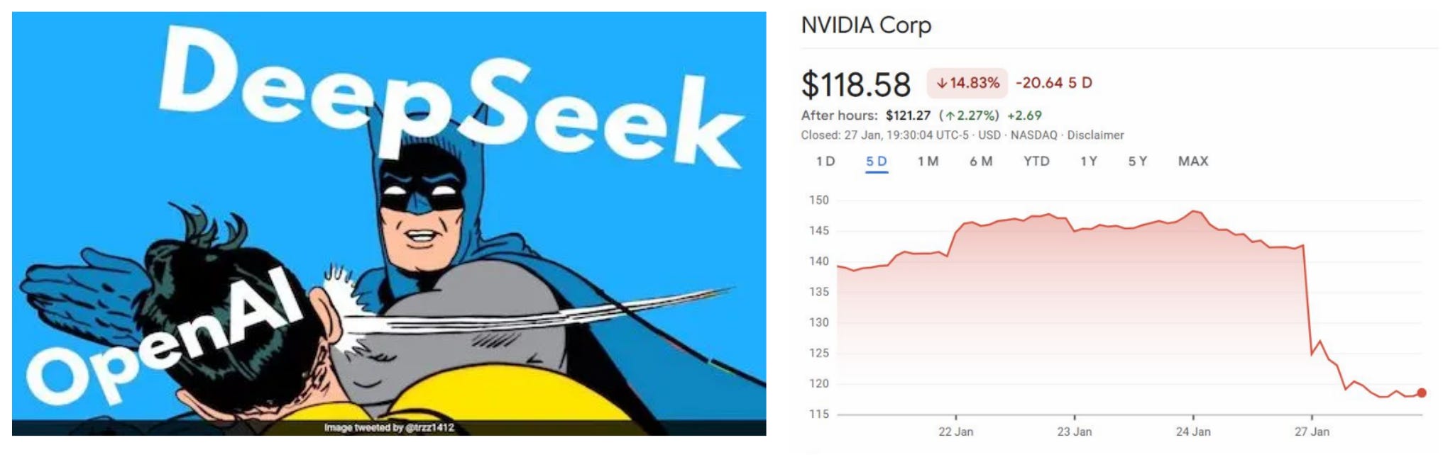
The moment constituted a powerful slap in the face to the prevailing view that expensive GPUs (promoted by NVIDIA) and high-budget models (like those from OpenAI) were indispensable for advanced AI:
👀 R1 demonstrated something the field had suspected but never proven at this scale: Great reasoning doesn’t require trillion-parameter models. Rather, it requires the right RL formulation.
Formalizing the Post-training Framework
DeepSeek-R1 is an RL post-training framework that helps LLMs acquire real reasoning ability purely through reinforcement learning without needing human-annotated reasoning traces.
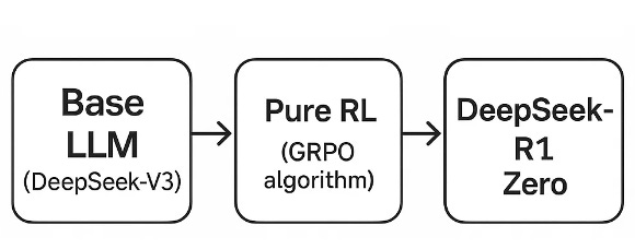
In the paper [1], the authors present 2 DeepSeek-R1 versions. In the original “R1-Zero” variant, the authors start from a base LLM (DeepSeek-V3-Base) and apply a pure RL pipeline with a verifiable final-answer reward (for math, code, STEM tasks) and without any supervised fine-tuning (SFT). Over thousands of training updates, the model begins to exhibit emergent reasoning behaviors: self-verification, chain-of-thought generation, reflection, and dynamic strategy adaptation.
The final, polished DeepSeek-R1 extends this with a multi-stage pipeline: a cold-start using a small curated CoT dataset to improve readability, followed by RL, then rejection-sampling to build fresh SFT data, then another RL pass (including domain-general prompts).
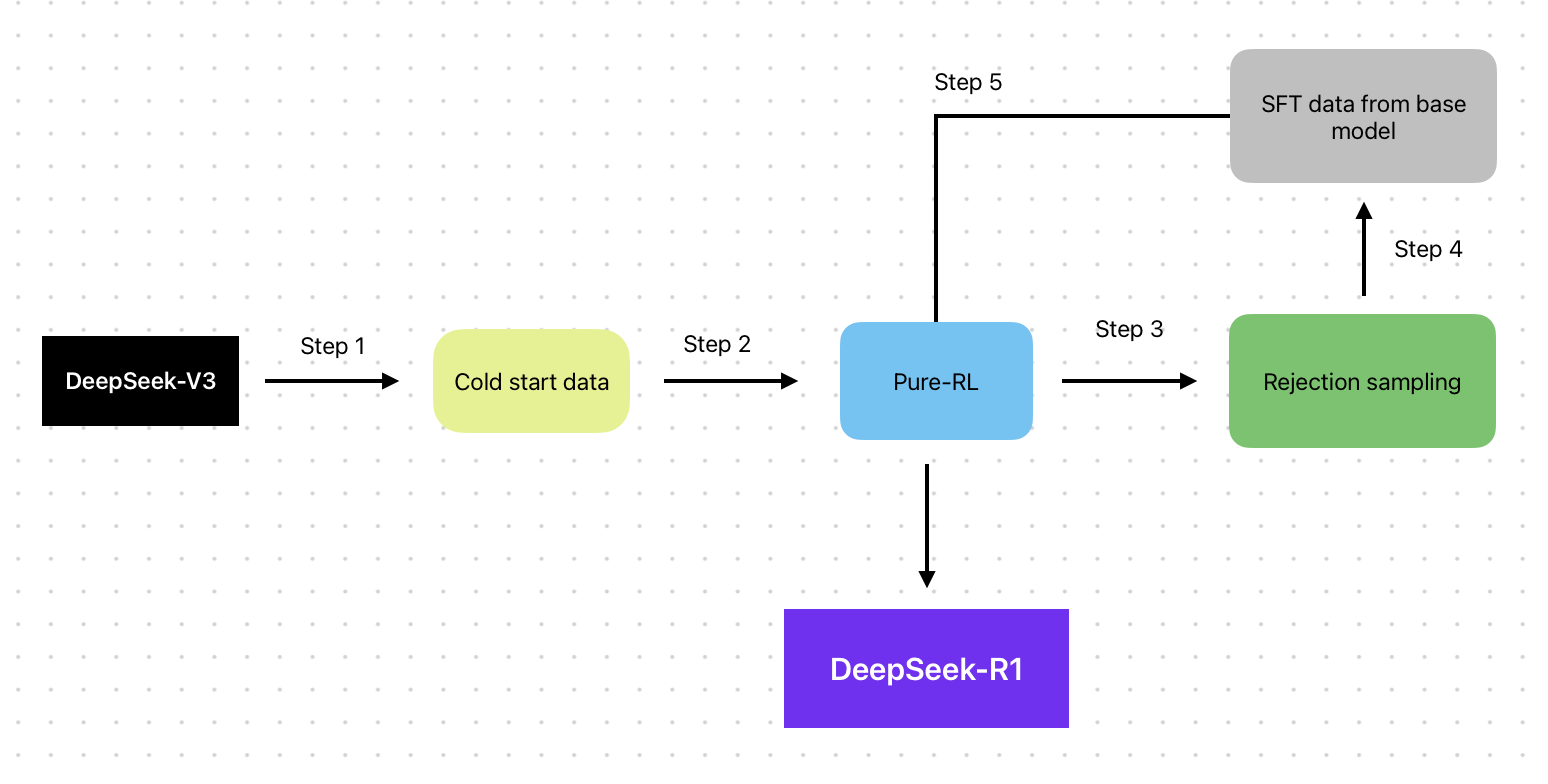
A key is what happens after the first RL run. DeepSeek takes the improved RL policy and uses it to generate many candidate reasoning traces for new problems. Instead of directly using the raw samples, they apply rejection sampling:
Keep only trajectories with correct final answers
Optionally rank by readability, coherence, or internal consistency
Discard the rest completely
This gives you a large dataset of high-quality, self-generated reasoning demonstrations. It’s like mining the model’s own best moments and discarding the noise.
👀 Crucially, this dataset is much cleaner than the original SFT data with no human variation, a fully standardized structure, and perfectly aligned with the target format introduced during warm-start.
Then, DeepSeek performs an SFT pass on the new data. This step accomplishes two things:
It distills the stable reasoning behaviors discovered during RL into a single, deterministic forward pass.
It smooths out the variance of RL sampling, making the model’s outputs cleaner and more consistent at inference.
At the end, the key component is the Pure-RL block. To understand it, we begin by framing LLM reasoning as an RL problem. An LLM acts as a conditional policy πθ over text, and each reasoning trajectory can be viewed within the standard RL tuple (S,A,R):
State st: the prompt q plus the partial generation up to step t:
Action at: the next token xt drawn from the policy:
Reward r: a final sequence-level reward given after the full output is completed:
where a* is the ground-truth answer, and R is the reward function that can measure how accurate the output x1:T is compared to the true answer a*. Usually, a simple exact match function with the ability to extract the final answer from the output is used. Because the reward is computed based on the ground-truth answer given by the dataset, it is:
✔️ Verifiable
✔️ Not requiring human annotations
This simple reward mechanism is crucial to DeepSeek-R1’s success, establishing it as an affordable alternative model. Yet, one question remains: 🧠 If the method is so straightforward, why has no one successfully implemented it before?
The answer lies in the RL, which demands specialized techniques to work effectively in the LLM context:
RL is Inherently Hard to Train: Standard RL algorithms are notoriously sample-inefficient and often exhibit high variance. Training requires meticulous tuning and robust techniques to stabilize the learning process.
Need for a Strong Base Model: RL algorithms typically cannot “bootstrap” a successful model from scratch. They require a “strong enough” base model to provide a solid foundation of language understanding and coherence. The base model used for DeepSeek-R1 (DeepSeek-V3), which is actually quite substantial and not small at all, provides this necessary strength to enable RL fine-tuning to work effectively.
Sparse Reward Problem: The task of aligning an LLM often results in a sparse reward signal. The model only receives feedback on the quality of its final response, making it difficult for the RL agent to determine which specific intermediate steps or tokens contributed to the success (or failure) of the output.
Necessity for a Novel RL Algorithm: Due to the issues of high variance and sparse rewards, the authors could not simply apply a naive or off-the-shelf RL technique. They had to adopt a new RL algorithm, named GRPO, specifically designed to be stable, scalable, and effective when applied to the vast parameter space of a powerful base LLM in a practical setting.
The RL Algorithm: Group-Based Policy Optimization (GRPO)
DeepSeek-R1’s RL algorithm is based on a well-known trust-region algorithm, called PPO [2]. To remind you, the original PPO objective is like this:
where wt is the important sampling ratio for action at.
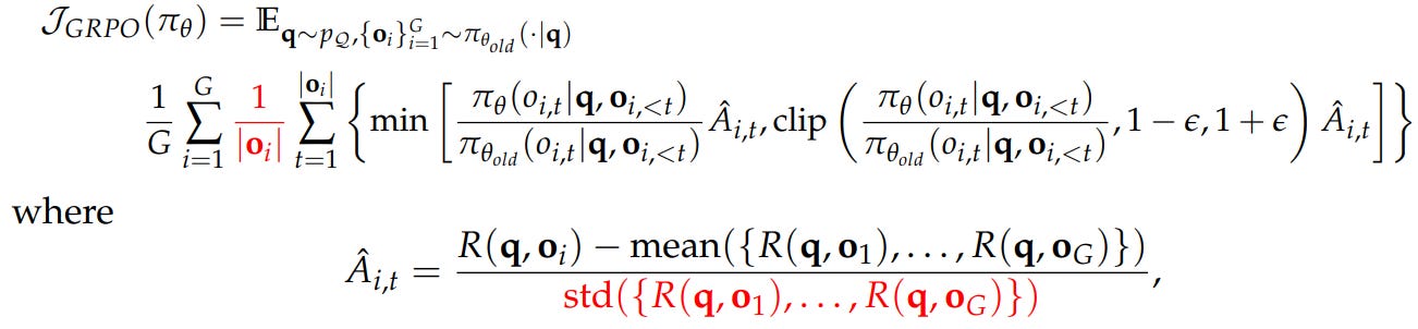
Here, DeepSeek-R1 modifies PPO with a group-based policy optimization scheme suitable for text space, which results in a new group-based advantage function. Specifically, for each query q, the model samples a group of G candidate outputs:
Each output oi represents the whole sequence of tokens and receives a scalar reward ri. Instead of fitting a value function and using the value function estimation in calculating the advantage, DeepSeek uses relative ranking inside the group to compute advantages:
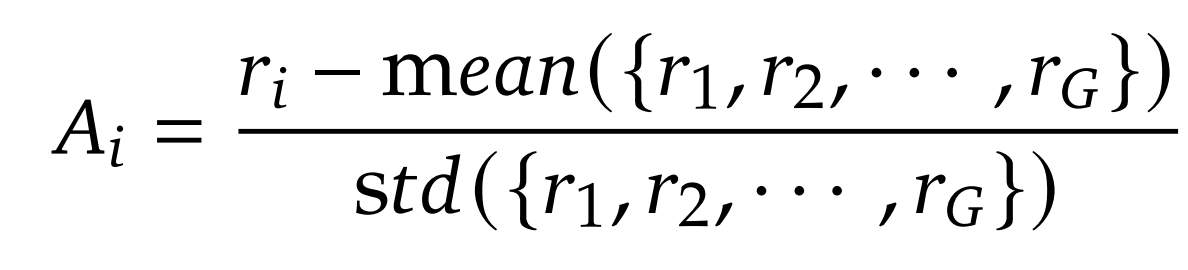
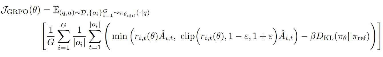
This yields a stable, variance-reduced advantage signal without a critic. The optimization objective is a PPO-style clipped surrogate, coupled with a KL constraint:
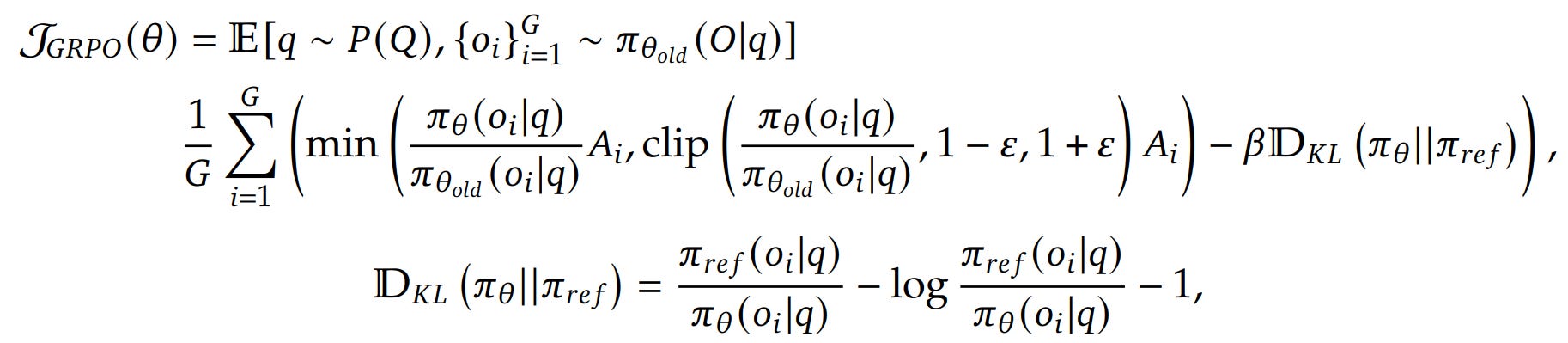
Here is the summary of GRPO’s features:
It operates on a whole sentence level, not a step/token level.
It avoids learning value networks and lets the reward signal directly shape reasoning behaviors through group-based advantage estimations.
The objective function is averaged over G outputs, reducing variance in the gradients
The DPO clip forces the update to be small, increasing stability.
The KL further forces the new LLM to be close to the base model, maintaining general pre-trained performance.
On the Reward Choice
As discussed earlier, the reward is simple and verifiable based on the ground-truth. However, to support reward calculation, the output of LLM must follow certain formats to allow later extraction of the final answers. If the model rambles, changes styles mid-generation, or forgets to delimit its conclusion, the verifier can’t score it, even if the reasoning is mostly correct. Therefore, DeepSeek-R1 proposes using the following prompt to ensure output format:
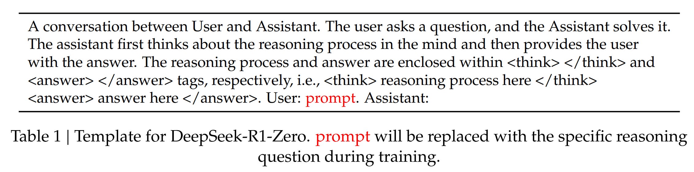
Once the output is parseable, the reward becomes a clean deterministic function:
where a is the extracted answer between <answer></answer> and a* is the true answer.
Other Interesting Insights
One of the most surprising findings is that you don’t need any chain-of-thought supervision to unlock multi-step reasoning. The model invents a reasoning style because it is the only reliable way to consistently maximize outcome reward. This is a major shift in thinking:
Reliable Answer⇒Reliable Internal Search
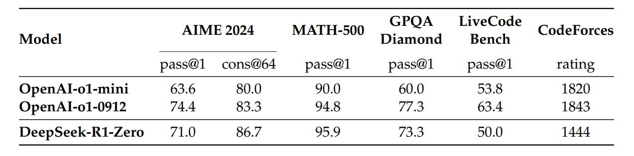
The model rediscovers analysis → checking → correction, not because we teach it, but because outcome reward makes messy one-shot answers unstable, failing to generalize to many input questions seen during training. As proved by the results, pure RL post-training is already competitive against other baselines:
Second, the paper also indicates the benefit of later SFT or distillation that compresses RL behaviors. After the first RL run, DeepSeek rejects low-quality samples and distills the remaining high-quality traces back into the model. You might expect a noticeable drop in performance because SFT is usually seen as “blurry” compared to RL. Instead, the distilled model actually becomes more stable and often more accurate.
Why? RL discovers a diverse set of good reasoning strategies, but SFT selects only the clean, high-confidence trajectories and forces the policy to reproduce them deterministically. The result is a smoother, more reliable reasoning model without the sampling volatility of pure RL.
👀 RL finds the behavior; SFT perfects it.
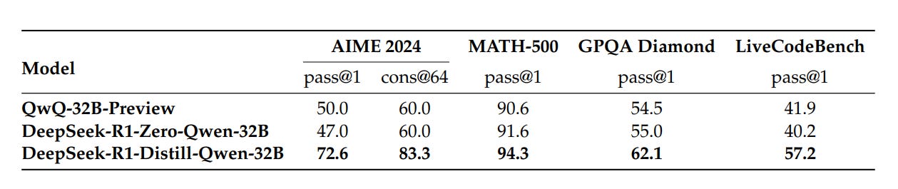
This approach of distillation from RL-trained big models to smaller ones is very effective:
Finally, one of the most striking aspects of DeepSeek-R1 is how much emergent structure arises even though the reward is extremely simple. There is no preference model, no human-written quality annotations, no chain-of-thought supervision baked into the reward. Yet the model discovers behaviors that look almost like they were explicitly trained for: the “aha moment”.
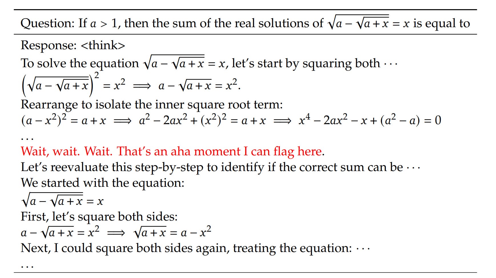
👀 Although the behavior is indeed interesting and never seen in training data, subsequent papers (e.g., in [3]) show that the base LLM intrinsically possessed this capability, though it manifested with a lower probability before fine-tuning.
Beyond GRPO: For A Better RL Post-Training
In the previous section, we saw how GRPO laid the foundation for post-training RL: by estimating advantages across sampled reasoning trajectories, GRPO reduces variance compared to naïve policy gradients and reliably nudges the model toward higher-reward outputs. However, it remains rudimentary and leaves plenty of room for improvement. GRPO is still rudimentary in several ways:
Residual variance in long reasoning chains: As tasks grow in complexity, the gradient signal from sampled trajectories can remain noisy, making learning slow or unstable.
Vulnerability to rare but correct trajectories: GRPO updates can inadvertently reduce the probability of correct but infrequent outputs, especially under sparse rewards.
Scalability bottlenecks: When applied to very large models or long, multi-step reasoning, GRPO can become computationally expensive and less stable.
Alternative RL Algorithms
To improve GRPO, many researchers have come up with alternative algorithms for RL post-training. For example, researchers introduced Decoupled Clip Dynamic Sampling Policy Optimization (👉DAPO [4]), which is a set of algorithmic and engineering fixes to make RL practical and reproducible at scale.
Trick 0: Remove KL term
Standard GRPO uses a KL penalty to constrain policy divergence. The authors exclude this term because long-CoT reasoning requires significant distributional shifts from the initial model, rendering the restriction unnecessary.
Trick 1: Clip-Higher
Recall that the clip in GRPO is to constrain the policy update, stabilizing the training. However, because of the constraints, standard clipping restricts probability updates: high-probability “exploitation” tokens can grow freely, but low-probability “exploration” tokens struggle. For example: with ε = 0.2 and positive advantage:
Token A: πθold=0.9 → upper bound 0.9⋅1.2=1.08
Token B: πθold=0.01 → upper bound 0.01⋅1.2=0.012
Here, high-probability tokens (A) easily increase, but rare tokens (B) barely move. This limits exploration and slows scaling. DAPO fixes this with the Clip-Higher strategy. Clip-Higher relaxes the upper bound for low-probability tokens, enabling more diverse sampling and helping the model discover better reasoning trajectories. In practice, the idea is implemented by simply modifying the clip part:
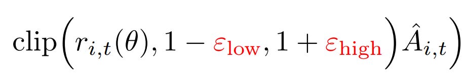
By using different hyperparameters for low and high clipping thresholds, the authors increase the value of εhigh to create space for the increase of low-probability tokens. while keeping εlow small because increasing it will drive these token probabilities toward zero, collapsing the effective sampling space.
Trick 2: Token-Level Policy Gradient Loss
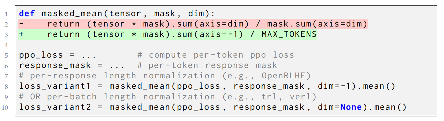
The original GRPO setup reduces the loss at the sample level: it calculates the probability of the whole response by averaging token probabilities within a sample, then averages across samples, giving every sample the same weight. In implementation, it looks like this:
Because the token contribution is normalized by the length of the response, tokens inside long responses effectively count less. This creates two issues:
Good long answers are undertrained, as the model can’t fully absorb the reasoning patterns in key tokens in the long answers.
Bad long answers are under-penalized as gibberish repetition isn’t punished strongly enough, causing entropy and response length to drift upward
To fix this, DAPO switches to a token-level policy gradient loss, giving each token its fair contribution to the update by not normalizing by response length but by the total number of tokens. The loss is:
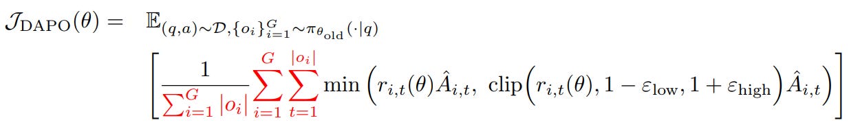
Under this formulation, longer sequences naturally exert more influence on the gradient than shorter ones. More importantly, useful token patterns, whether they appear early or deep inside the reasoning trace, are updated proportionally, and harmful patterns get penalized no matter where they occur.
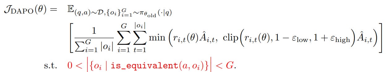
Trick 3: Dynamic Sampling
A subtle issue in GRPO-style algorithms is that when a prompt’s outputs all achieve 100% accuracy, every sample in that group receives the same reward. This collapses the advantage to zero, leading to zero gradients, which means weaker updates, higher noise sensitivity, and degraded sample efficiency.
Worse, as training progresses, the number of “all-correct” prompts steadily increases, so the effective number of learning prompts per batch shrinks. DAPO addresses this by oversampling and filtering prompts whose accuracy is exactly 1 or 0. Only prompts with meaningful gradient signals are retained, ensuring every batch contains a stable number of informative prompts. Before each update, the system dynamically samples until the batch is fully populated with prompts that provide non-zero gradient contribution, keeping training stable even as accuracy improves.
Trick 4: Overlong Reward Shaping
Most RL pipelines cap the maximum generation length and simply truncate responses that run past it. The default practice is to assign a punitive reward to these truncated samples. But in long-CoT reasoning, this turns out to be harmful: a perfectly good chain of thought may get cut off just because it’s long, and the model is punished for the wrong reason.
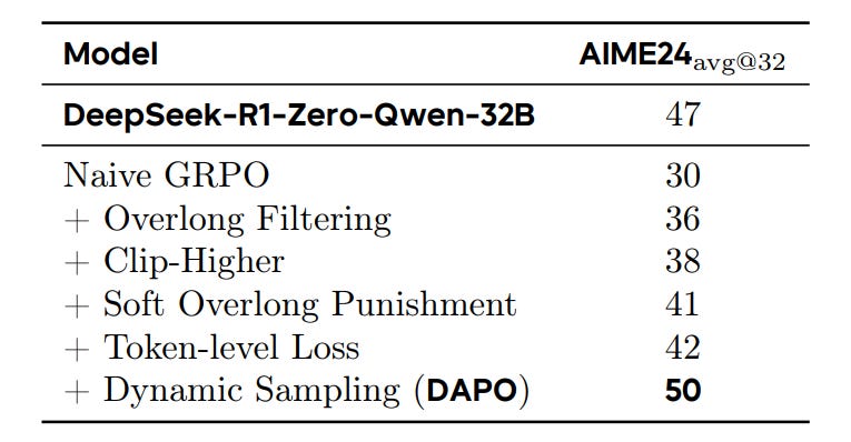
DAPO proposes to mask the loss of truncated outputs (Overlong Filtering), making training dramatically more stable and performance on benchmarks like AIME jumps immediately. But filtering alone isn’t enough. Long responses can still waste tokens and reduce efficiency. So DAPO introduces a Soft Overlong Punishment, a gentle, length-aware shaping term:
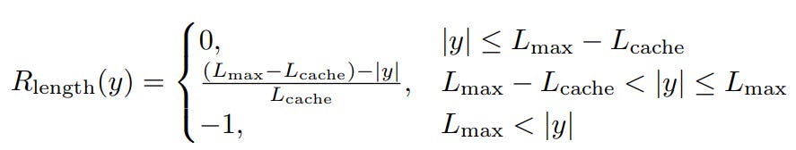
This function grades the penalty smoothly as the model approaches the max-length zone, which is Lcache from Lmax, and only applies a full −1 reward when it exceeds Lmax.
The result is incrementally better as we apply these tricks one by one:
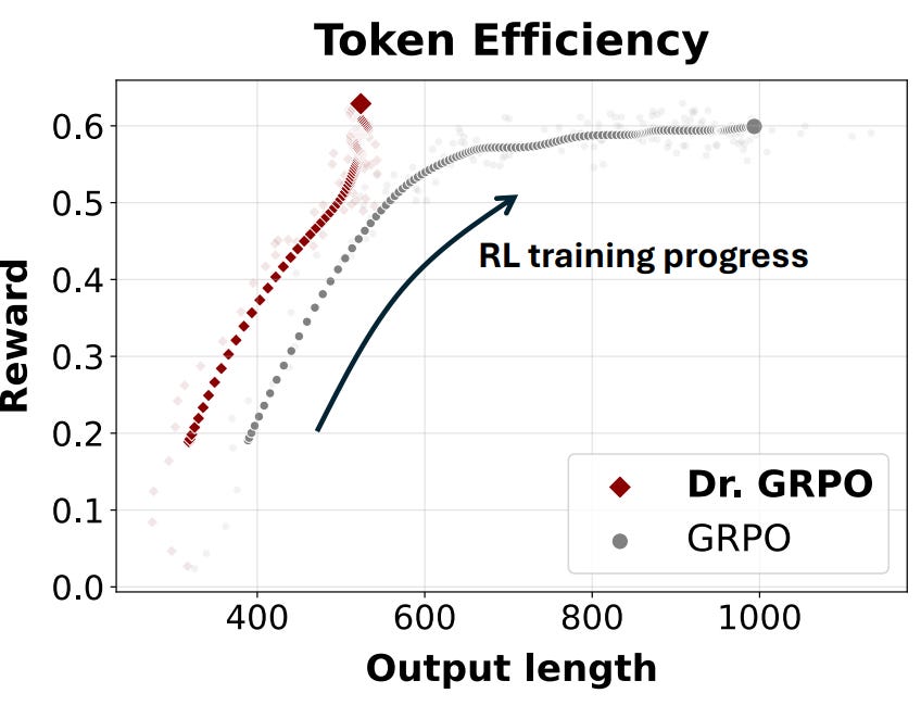
At the same time, concurrent researchers have started investigating other changes to the GRPO algorithm. Paper 👉Dr. GRPO [5] reveals 2 limitations of GRPO as a result of dividing the advantage by response length and per-question return variance.
Both seem harmless at first glance, but together they create two systematic biases:
❌ Length bias: If a response is correct, shorter outputs get larger gradients because you’re dividing a positive advantage by fewer tokens. If a response is incorrect, longer outputs get less penalty because they’re cushioned by a bigger length divisor. Over time, this pushes the policy toward long incorrect chains and short correct ones. Simple fix:
👀 This is similar to the token-level policy loss trick in DAPO paper.
❌ Difficulty bias: Normalizing by the per-question standard deviation means that questions where all responses are almost correct (or almost wrong) get disproportionate weight. Easy or impossible examples dominate updates, while medium-difficulty ones, where reasoning actually matters, get suppressed. This can be simply fixed by removing the std denominator:

These tricks accelerate the progress of RL post-training:
In addition to the above simple tricks, other papers look for fundamental changes to the RL algorithm. One of the big limitations of pure on-policy RL for reasoning (GRPO/PPO-style) is that the model can only explore what it can generate. If the base model can’t produce high-quality chains of thought, then RL mostly just amplifies its existing bias patterns instead of teaching it genuinely new reasoning skills.
The paper, Learning to Reason under Off-Policy Guidance (👉LUFFY [6]), introduces a simple but surprisingly effective idea: use off-policy guidance such as reasoning traces from a much stronger model (e.g., DeepSeek R1), and fold them directly into the RL pipeline so the learner can “see” good reasoning even before it can generate any. But unlike naïve imitation, the goal here is not to copy the teacher; it’s to blend demonstrations into GRPO in a way that preserves exploration and lets the student ultimately outgrow the off-policy samples.
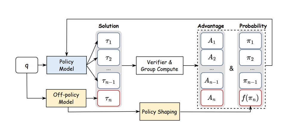
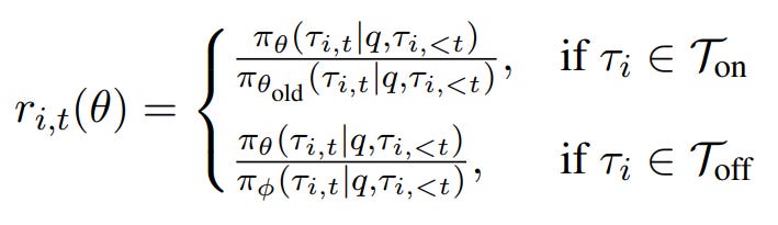
Formally, let Gon and Goff denote on-policy and off-policy trajectory groups, sampled from πθold and πϕ, respectively. LUFFY computes advantages using the union of both:
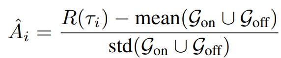
This ensures that high-quality off-policy trajectories receive larger advantages early in training (as on-policy rollout is worse), accelerating learning without overriding on-policy exploration as the policy improves. Then, two PPO-styled objectives for on- and off-policy training are used to update the current policy. Here, the off-policy term uses its own importance sampling ratio:
Together, we have a mixed objective:
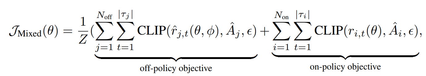
where Z is the total number of tokens, serving as a normalization term.
👀 Because πθ is much closer to πθold than to πϕ, the off-policy ratio gradually becomes smaller, naturally tempering gradients from the off-policy data.
Now, one problem arises. Naively mixing off-policy data leads to rapid entropy collapse: the model overcommits to high-probability actions that coincide with off-policy tokens, eliminating exploratory behaviour required for multi-step reasoning. To counter this, LUFFY applies a shaping transformation to the off-policy importance ratio f(r) and removes the clip function, yielding the shaped off-policy gradient:
If we derive the gradient contribution for each candidate off-policy token τ′t at time t:
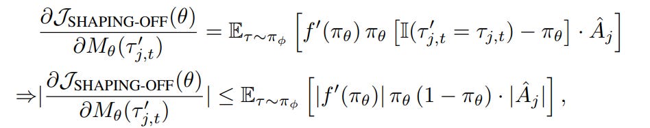
If we don’t use the shaping function, f(r) = r, f’(r)=1, then the gradient magnitude is bounded by πθ(1−πθ). This term is tiny when:
πθ is near 0 → model thinks the token is impossible
πθ is near 1 → model is already confident
This is bad because the model struggles to get gradient signals from new reasoning moves (often starting with low-probability tokens). Thus, they propose shaping a function like this:
where γ is set as 0.1. This has the key effect:
When πθ is small, f′ is large⇒boosts gradients
When πθ is large, f′ shrinks⇒dampens near-certain tokens
This improves the exploration and avoids entropy collapse:
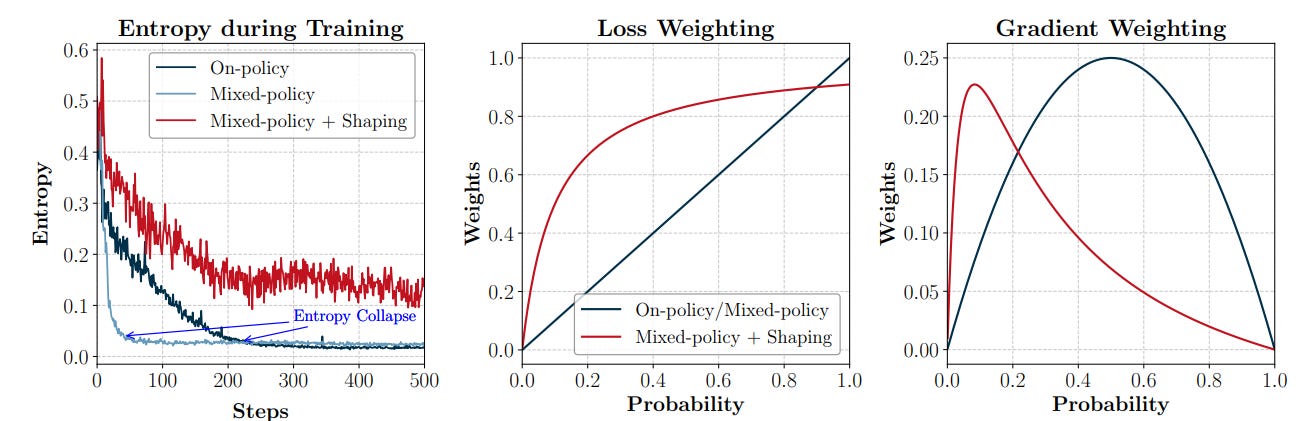
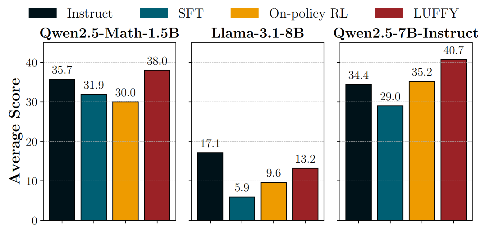
and better performance overall:
Reward Shaping
Improving the RL algorithm is only part of the story. The other part is how we tell the model what success looks like. Reward design shapes the entire search landscape that the model explores. A good reward doesn’t just score outputs; it pulls the model toward the kinds of internal reasoning moves we want it to adopt. And unlike test-time scaling, reward shaping changes the model’s internal dynamics, not just its decoding strategy. The right reward can turn a passive pattern-matcher into an active problem-solver.
One important element in determining reasoning quality is the CoT length: Give models more thinking time, and they often reason better. But when you fine-tune a model on long-form CoT traces and then optimize it with RL, the model doesn’t merely preserve the long patterns; it tends to amplify them. Both Llama-3.1-8B and Qwen-2.5-Math-7B quickly push their CoTs longer and longer until they hit the context limit. Once trajectories exceed the max length, the model gets a negative or zero reward, not because the reasoning is bad, but because the sequence literally doesn’t fit.
👀 Similar problem like Trick 4 in the DAPO paper.
To fix this, the authors propose a length-based reward shaping, named 👉Cosine Reward [7]. It introduces a very clean idea: make the reward sensitive to the CoT length.
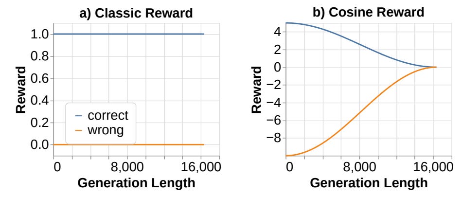
Instead of the classic “1 for correct, 0 for incorrect” sparse reward, they use a piecewise cosine reward that encodes three simple principles:
Correct > wrong: Correct answers always get a higher reward than wrong ones.
Shorter > longer (if correct): Among correct solutions, shorter CoTs are better.
Longer > shorter (if wrong): If the model is wrong, encourage it to think longer next time.
To implement this, they propose a reward formula:
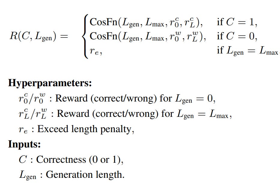
where:
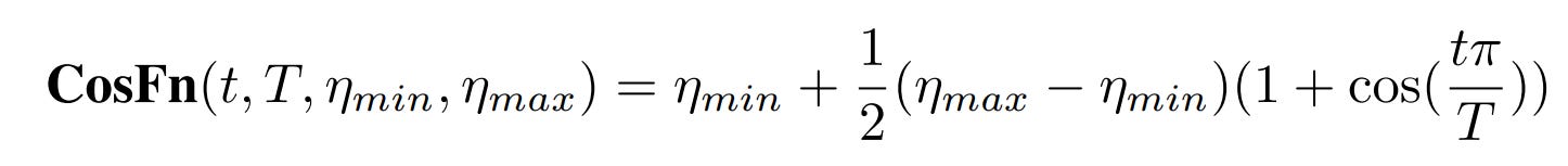
This function makes sure that as Lgen increases to Lmax, the reward smoothly changes between the two reward hyperparameters. Depending on the correctness, the reward change can be decreased (correct) or increased (incorrect):
The addition of Cosine Reward to RL training helps stabilize training as the number of training iterations increases:
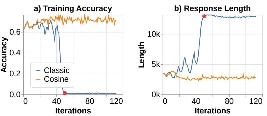
👀 As we will see later, the drop of performance due to repoonse length suddenly jumps to max is one of the “training collapses“ often occured in RL post-training.
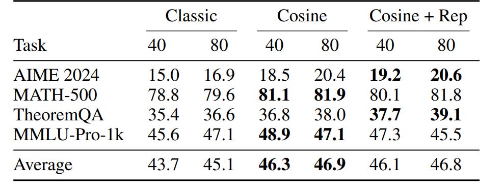
However, introducing a length-based reward like Cosine Reward can be problematic. As for incorrect answers, a longer response is encouraged. The model exhibited reward-hacking behavior, inflating CoT length on difficult problems through repetition rather than genuine reasoning.
To address this, the authors introduce an N-gram repetition penalty: apply token-level penalties directly at the positions where repetition occurs. By recording N-grams at every step, they can detect an N-gram repetition to add a penalty (as a negative reward, for instance).
These reward shaping techniques collectively help improve the reasoning performance on math datasets significantly:
As we can see, length-aware reward shaping helps stabilize emergent CoT scaling by nudging models toward efficient reasoning trajectories. However, even sophisticated length-based rewards face a key limitation: they assume the model is already capable of producing coherent, partially correct reasoning. This assumption breaks down for weaker models such as tiny LLMs(≤1B parameters), where reasoning is fragile, and outcome rewards are extremely sparse. This leads to a natural question: 🧠 How do we guide RL training when the model fails to produce any correct trajectories for long periods of time?
This is where the 👉Memory-R+ [8] paper contributes a major new idea:
Memory-augmented intrinsic rewards. The Memory-R+ method proposes a shift in perspective: instead of relying solely on external rewards (correct/incorrect), the model should also learn from its own past reasoning, much like humans rely on episodic memory.
The approach introduces two episodic memory banks:
Success Memory (Mₛ): stores reasoning traces that led to the correct answer
Failure Memory (Mf): stores reasoning traces that produced incorrect results
These memories are stored as embeddings in a shared representation space using a Sentence Transformer encoder. The key idea is simple but powerful:
Reward the model when its reasoning resembles past successes
Reward the model when it avoids past failures
This creates a dense, performance-driven intrinsic reward signal that tiny models desperately need. Given a new query, the memory system:
Looks up similar past queries in both success and failure memories using k-NN in embedding space.
Retrieves the associated reasoning traces (not just final answers).
Evaluates the new response based on:
similarity to successful reasoning (exploit)
dissimilarity to failed reasoning (explore)
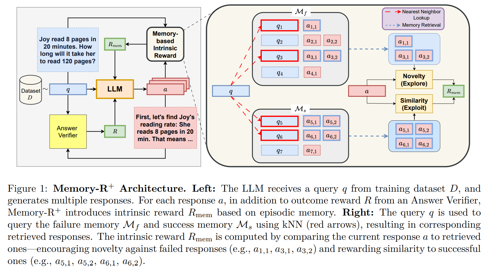
Exploit Reward
The success memory provides a set of retrieved successful reasoning traces B. Their embeddings are averaged to form a centroid:
A generated response a earns a higher reward when it is closer to this centroid:
This encourages generalizable reasoning patterns, not rote memorization.
It captures structure like “identify quantities → set up equation → solve”, even if the surface text differs.
Explore Reward
Failure memory provides a set of incorrect reasoning traces. The authors measure novelty as the inverse similarity to the closest failure:
If the model repeats a failed reasoning pattern, its reward goes down. If it proposes a novel direction, the reward goes up. This creates a natural curriculum:
Early: encourages broad exploration (most reasoning is wrong).
Later: focuses on fine-grained distinctions between near-correct and correct reasoning.
Finally, each intrinsic reward is min-max normalized over a sliding window, then combined:
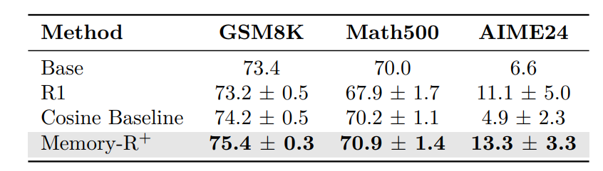
The results are improvements across many tiny LLMs, including one with Thinking Mode (Qwen3-0.6B):
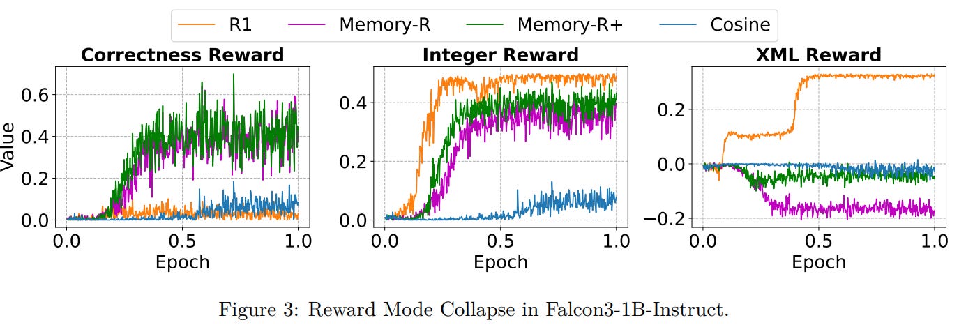
Training Instability and Collapse in LLMs
The paper also analyzes the training collapse issues with RL post-training. LLMs often over-optimize simpler rewards, such as format rewards, at the expense of correctness, a phenomenon known as reward mode collapse. Models without intrinsic rewards focus on easy metrics, while Memory-R+ balances exploitation (aligning with successful reasoning) and exploration (avoiding past failures), preventing collapse.
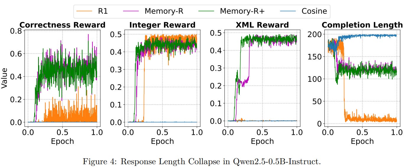
Response length collapse is another issue: models either under-generate (too short) or over-generate (too long) sequences, producing meaningless outputs. Length-based rewards like Cosine can worsen this. Memory-R+ stabilizes training by providing dense memory-based feedback, ensuring reasonable response lengths while improving correctness.
While Memory-R+ effectively stabilizes tiny LLM training through episodic memory and intrinsic rewards, it primarily operates at the response level, assigning rewards based on entire reasoning chains or key intermediate patterns. However, recent research has highlighted the benefits of dense process rewards that provide feedback at each reasoning step, rather than only at the outcome.
👀 Token- or step-level feedback allows the model to understand which intermediate decisions are correct, improving training efficiency and reasoning fidelity.
Despite their advantages, dense rewards are rarely deployed at scale in RL for LLMs. The challenges are threefold:
❌ Defining process rewards: Assigning meaningful credit to intermediate steps is non-trivial, as some seemingly “incorrect” steps may contribute indirectly to a correct final answer.
❌ Scalability of online updates: Updating dense reward models (process reward models, PRMs) online requires frequent retraining on step-level labels, which is costly and often infeasible.
❌ Extra modeling cost: Conventional dense reward methods require separate reward models trained with expensive annotations, adding significant overhead.
The 👉PRIME [9] framework (Process Reinforcement through Implicit Rewards) offers an elegant solution. Instead of requiring step-level labels, PRIME leverages implicit process reward modeling to generate token-level dense rewards derived from standard outcome labels. Essentially, a single reward model can infer dense rewards for each step, which are updated online with policy rollouts. This approach:
✔️ Provides fine-grained, step-level feedback for improved credit assignment.
✔️ Reduces reward sparsity without additional annotation cost.
✔️ Mitigates reward hacking by updating the reward model along with the policy, maintaining alignment between the model and its reward signal.
The Implicit PRM is trained only with outcome-level labels but can produce token-level dense rewards. To be specific, the reward model πϕ is trained with the outcome reward:
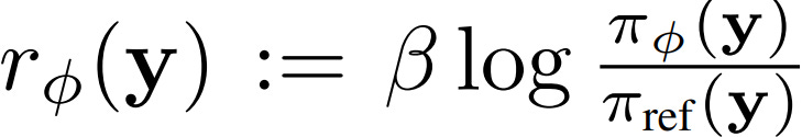
We can train it using cross-entropy loss (after applying the sigmoid function to normalize the reward) based on whether the output is correct or not, such that sequences with higher outcome rewards should be assigned a higher reward.
Then, during inference to generate dense rewards for RL post-training, the reward at step t (i.e., for token yt) is:
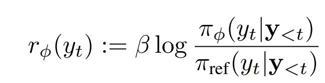
where:
πϕ = the Implicit PRM (reward model)
πref = reference model (often the initial SFT or base LM)
β = scaling factor
👀 The reward measures how much more likely the PRM is to generate this token compared to the reference model, which implicitly reflects intermediate correctness or quality at that token.
Because we now have a reward for every step, we need to calculate the advantage function used in the RL algorithm (not necessarily GPO). Here, they propose to use a leave-one-out (LOO) baseline, resulting in the advantage function for each step t:
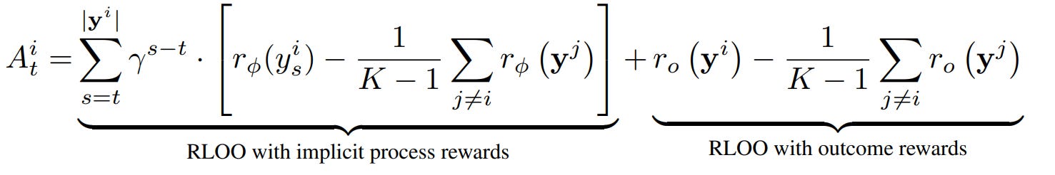
The advantage consists of the implicit process reward and outcome reward components. With a step-based advantage, they can use the standard step-level PPO as the RL objective:
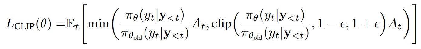
❌ However, training an additional reward model and using step-level PPO can be computationally expensive.
Optimizing the Training Pipeline
So far, most advances in post‑training RL for reasoning optimize which algorithm to use or how to shape the reward. But there’s a third: how we structure the training itself, e.g., via curriculum learning. Curriculum learning is inspired by human education: instead of exposing a model to the hardest tasks from the start, we begin with easier tasks and progressively increase difficulty. So the key task is to estimate the difficulty of the data sample.
In the 👉AdaRFT [10] paper, the authors propose to use precomputed difficulty scores for each problem, which can come from human annotations, empirical success rates, or a separate difficulty-estimation mode. For example, they use an external LLM as the difficulty estimator. The problem now is choosing the right estimator model because not all models are suitable for difficulty estimation:
Too strong (e.g., OpenAI o1, DeepSeek-R1): These models solve most problems on the first attempt, leaving little variance across problems. As a result, easy and hard problems cannot be distinguished effectively.
Too weak (e.g., LLaMA 3 1B): These models fail on nearly every problem, producing insufficient signal to guide curriculum adaptation.
Thus, they select Qwen 2.5 MATH 7B as the difficulty estimator because it exhibits balanced problem-solving ability: it succeeds on moderately difficult problems but struggles with the most challenging ones. Then, for each problem i, the difficulty score di is defined as:
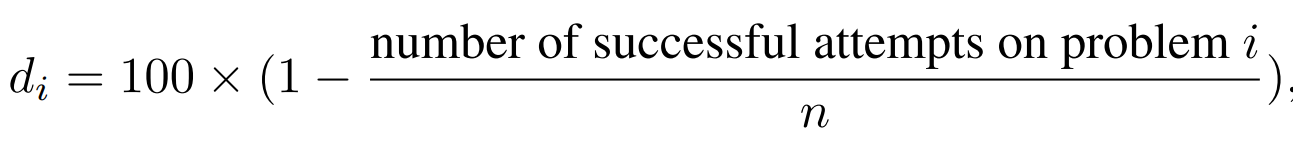
This represents the empirical average accuracy of the estimator on problem i. With the difficulty score, the curriculum goal is to assign the samples with difficulty most suitable to the current model (target difficulty), not too easy, not too hard. As such, starting with an initial level of difficulty target, as the LLM improves over time, the target difficulty increases; if performance drops, it decreases. At each step, the model is finetuned on problems closest to the current target difficulty, ensuring steady, aligned progression. This is how it works in RL post-training:
Dynamic Curriculum Sampling
Compute the absolute difference between each problem’s difficulty and the current target difficulty.
Select a batch of problems that are closest to the target, keeping tasks neither too easy nor too hard.
Policy Update
The policy model generates responses for the selected batch.
Compute rewards based on correctness and update the policy using a reinforcement learning algorithm (e.g., PPO, GRPO, REINFORCE++).
Target Difficulty Update
The average reward over the batch determines whether to increase or decrease the target difficulty.
Smooth updates are ensured using a tanh function, while the difficulty is clipped within valid bounds.

👀 This algorithm introduces many hyperparameters, which can be problematic for tuning.
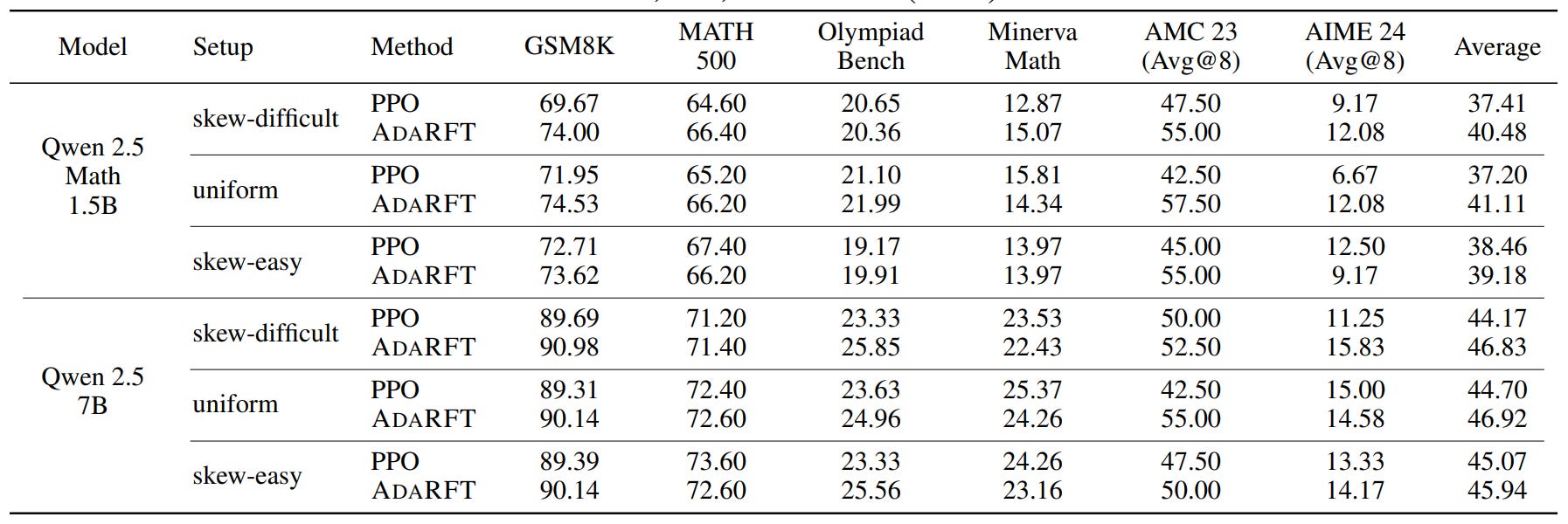
That said, the results have improved significantly:
In addition to difficulty estimation via external models, there can be a simpler way to define sample difficulty: rely on the length of the question. In the 👉FASTCURL [11] paper, the researchers analyze the DEEPSEEK-R1-DISTILL-QWEN-1.5B model and discover that longer input prompts generally produce longer output responses:
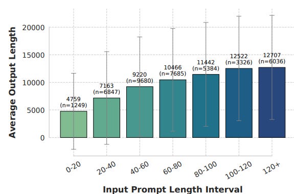
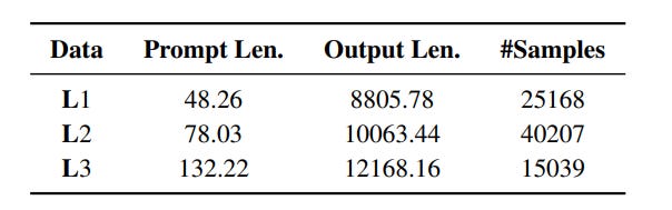
This observation motivated a simple but effective hypothesis: For complex reasoning tasks, the complexity of a problem correlates with the length of the solution the model must generate. Using this principle, the paper divides the training dataset into three subsets based on average input prompt length:
L1: Short CoT reasoning problems (simpler tasks, easy)
L2: The original dataset (baseline tasks, medium)
L3: Long CoT reasoning problems (more complex tasks, hard)
Below are the statistics of the datasets:
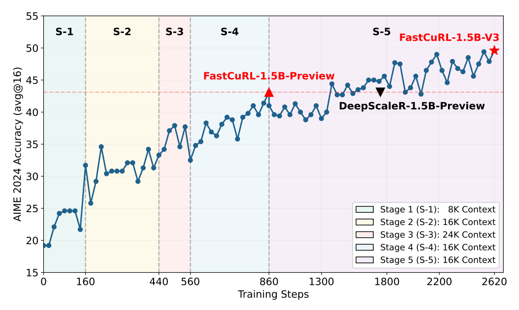
Therefore, the paper proposes to divide training into stages that correspond to different context lengths and data set lengths (difficulties). They tested with many configurations and found many good strategies. For example, they use 5 training stages corresponding to:
Context length: 8K, 16K, 24K, 16K, 16K
Datasets: L1, L2, L3, L2, L2
The intuition is first to progress from easy to hard (L1 to L3), then come back to the medium difficulty (L2) until convergence. No theory is given, but empirically, it works best:
Despite these good results, two major obstacles limit LLM performance in the normal curriculum setting:
❌ Difficulty Shift: In education science, there is a Difficulty Shift phenomenon, a.k.a., the model’s perception of a problem’s difficulty changes dynamically as it learns. A problem considered “hard” initially may become “easy” later, making a static difficulty score, as in AdaRFT or FastCuRL, obsolete.
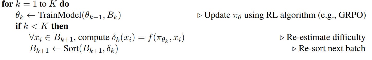
Inspired by this principle, the paper 👉ADCL+EGSR [12] focuses on optimizing the data progression via a dynamic data assignment. There are two contributions in the paper: ADCL and EGSR, where the former focuses on curriculum improvement and the latter helps with training guidance. First, instead of using a static task ordering, ADCL periodically re-estimates the difficulty of upcoming batches based on the model’s current state:
Initially, difficulty scores δ0 are assigned to all samples in the dataset D using the base model parameters θ0.
The dataset is sorted by these scores and partitioned into sequential batches B1,B2,...,BK.
After training on batch Bk, the model parameters are updated to θk.
ADCL re-evaluates difficulty scores δk+1 for the next batch’s samples and re-sorts the batch internally according to the new difficulty estimation before proceeding to the next iteration
Besides curriculum training, the paper also aims to address one issue of current RL post-training:
❌ On-Policy Exploration Limits: Standard post-training, rely solely on self-generated trajectories. While this can improve problem-solving for tasks the model can occasionally solve, it struggles when the model’s current knowledge is insufficient to produce non-zero reward outputs. This “zero-reward” scenario halts learning because gradient updates vanish, i.e., no signal for training.
To address this issue, they propose to incorporate training trajectories generated from an expert policy. This idea is very similar to the aforementioned LUFFY paper. However, instead of following the correct way of defining important sampling for on and off-policy data like this:
The paper indicates that directly using an expert policy πϕ is often impractical. The expert policy may be inaccessible or rely on incompatible tokenization, making probability ratio calculations infeasible. Even when available, the distributional mismatch between πϕ and the current policy πθold can result in extreme importance weights, leading to unstable updates. So they instead use expert demonstrations to guide the current policy in generating improved trajectories:
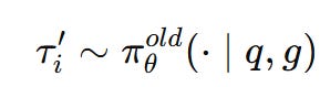
Here, the expert demonstration g is used in the prompt. This leads to a different training objective:
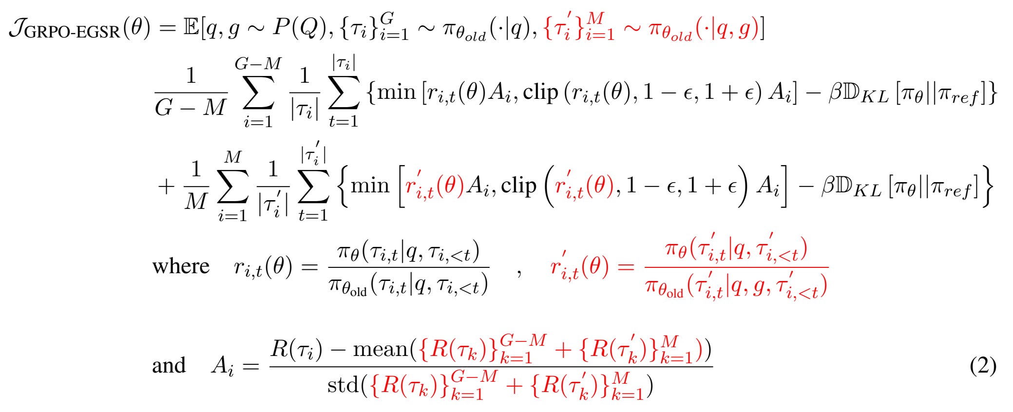
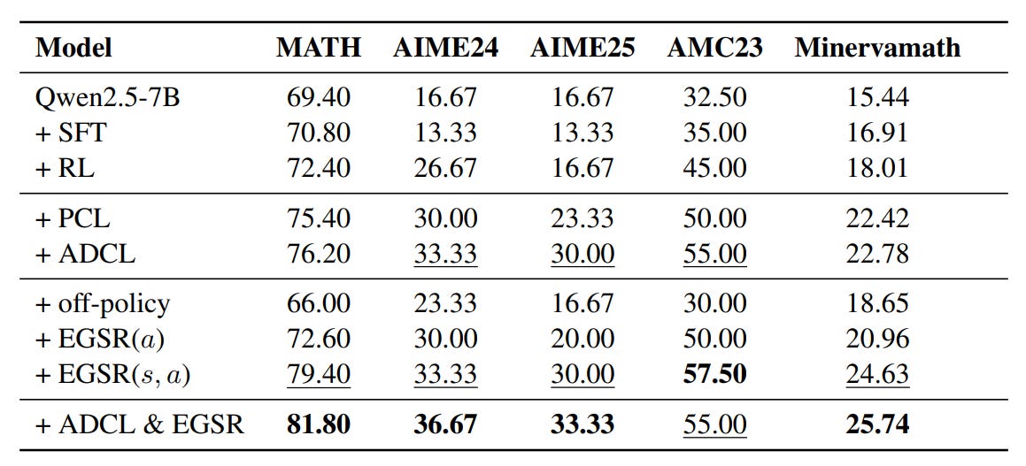
Here, the offline trajectories are generated by πθold, and the important sampling ratio for offline trajectories is now not significantly different from that for online trajectories. The advantages are also mixed between the two online and offline returns, as expected. The performance of the final model, ADCL+EGSR, is better than the standard RL post-training:
❌ A big limitation of the approach is that ADCL requires recomputing the difficulty scores for each sample frequently, which slows down training.
🧠 The question of how to build an efficient adaptive RL curriculum during LLM post-training remains open and calls for continued research [13].
References
[1] Guo, D., Yang, D., Zhang, H. et al. DeepSeek-R1 incentivizes reasoning in LLMs through reinforcement learning. Nature 645, 633–638 (2025). https://doi.org/10.1038/s41586-025-09422-z
[2] Schulman, John, Filip Wolski, Prafulla Dhariwal, Alec Radford, and Oleg Klimov. “Proximal policy optimization algorithms.” arXiv preprint arXiv:1707.06347 (2017).
[3] There May Not be Aha Moment in R1-Zero-like Training — A Pilot Study. https://sail.sea.com/blog/articles/62
[4] Yu, Q., Zhang, Z., Zhu, R. et al. (2025). DAPO: An open-source LLM reinforcement learning system at scale. NeurIPS 2025.
[5] Liu, Zichen, Changyu Chen, Wenjun Li, Penghui Qi, Tianyu Pang, Chao Du, Wee Sun Lee, and Min Lin. “Understanding r1-zero-like training: A critical perspective.” COLM 2025.
[6] Yan et al. (2025). Learning to Reason under Off-Policy Guidance. NeurIPS 2025.
[7] Yang, S., Tong, Y., Niu, X., Neubig, G., & Yue, X. (2025). Demystifying Long Chain-of-Thought Reasoning. In Proceedings of the 42nd International Conference on Machine Learning (ICML 2025).
[8] Hung Le, Van Dai Do, Dung Nguyen, and Svetha Venkatesh. Reasoning Under 1 Billion: Memory-Augmented Reinforcement Learning for Large Language Models. Transactions on Machine Learning Research (TMLR), 2025.
[9] Cui, Ganqu, Lifan Yuan, Zefan Wang, Hanbin Wang, Yuchen Zhang, Jiacheng Chen, Wendi Li et al. “Process reinforcement through implicit rewards.” arXiv preprint arXiv:2502.01456 (2025).
[10] Shi, Taiwei, Yiyang Wu, Linxin Song, Tianyi Zhou, and Jieyu Zhao. “Efficient reinforcement finetuning via adaptive curriculum learning.” arXiv preprint arXiv:2504.05520 (2025).
[11] Song, M., Zheng, M., Li, Z., Yang, W., & Luo, X. FastCuRL: Curriculum Reinforcement Learning with Stage-wise Context Scaling for Efficient Training R1-like Reasoning Models. Findings of the Association for Computational Linguistics: EMNLP 2025.
[12] Zhang, E., Yan, X., Lin, W., Zhang, T., & Lu, Q. Learning Like Humans: Advancing LLM Reasoning Capabilities via Adaptive Difficulty Curriculum Learning and Expert-Guided Self-Reformulation. EMNLP 2025.
[13] Do, Dai, Manh Nguyen, Svetha Venkatesh, and Hung Le. “SPaRFT: Self-Paced Reinforcement Fine-Tuning for Large Language Models.” arXiv preprint arXiv:2508.05015 (2025).
Brilliant deep dive into RL post-training. The GRPO insight about bypassing value networks entirely through group-based advantages is genius, it sidesteps the classic actor-critic variance problem that's plagued RL at scale. What's particualrly interesting is how this connects tothe sparse reward challenge: by ranking within groups rather than fitting global value functions, the model gets sharper feedback even when most trajectories fail. That relative comparison mechanism feels more robust than absolute reward estimation.